An Automatic System to Discriminate Malignant from Benign Massive Lesions on Mammograms

Abstract

Mammography is widely recognized as the most reliable technique for early detection of breast cancers. Automated or semi-automated computerized classification schemes can be very useful in assisting radiologists with a second opinion about the visual diagnosis of breast lesions, thus leading to a reduction in the number of unnecessary biopsies. We present a computer-aided diagnosis (CADi) system for the characterization of massive lesions in mammograms, whose aim is to distinguish malignant from benign masses. The CADi system we realized is based on a three-stage algorithm: a) a segmentation technique extracts the contours of the massive lesion from the image; b) sixteen features based on size and shape of the lesion are computed; c) a neural classifier merges the features into an estimated likelihood of malignancy. A dataset of 226 massive lesions (109 malignant and 117 benign) has been used in this study. The system performances have been evaluated terms of the receiver-operating characteristic (ROC) analysis, obtaining $A_{z}=0.80\pm 0.04$ as the estimated area under the ROC curve.

Keywords: Computer-aided diagnosis, Breast cancer, Massive lesions, Segmentation, Neural networks.

Introduction

Breast cancer is still one of the main causes of death among women, despite early detections have recently contributed to a significant decrease in the breast-cancer mortality [1, 2]. Mammography is an effective technique for detecting breast cancer in its early stages [3]. Once a massive lesion is detected on a mammogram, the radiologist recommends further investigations, depending on the likelihood of malignancy he assigns to the lesion. However, the characterization of massive lesions merely on the basis of a visual analysis of the mammogram is a very difficult task and a high number of unnecessary biopsies are actually performed in the routine clinical activity. The rate of positive findings for cancers at biopsy ranges from 15% to 30% [4], i.e. the specificity in differentiating malignant from benign lesions merely on the basis of the radiologist’s interpretation of mammograms is rather low. Methods to improve mammographic specificity without missing cancer have to be developed. Computerized method have recently shown a great potential in assisting radiologists in the visual diagnosis of the lesions, by providing them with a second opinion about the degree of malignancy of a lesion [5, 6, 7].

The computerized system for the classification of benign and malignant massive lesions we describe in this paper is a semi-automated one, i.e. it provides a likelihood of malignancy for a physician-selected region of a mammogram.

This paper is structured as follows: a technical description of the method is given in sec. 1; section 2 illustrates the dataset of mammograms we used for this study and sec. 3 reports on the performances the CADi system achieved in differentiating malignant from benign massive lesions.

1 Description of the CADi system

The system for characterizing massive lesions we realized is based on a three-stage algorithm: first, a segmentation technique extracts the massive lesion from the image; then, several features based on size, shape and texture of the lesion are computed; finally, a neural classifier merges the features into a likelihood of malignancy for that lesion.

1.1 Segmentation

Massive lesions are extremely variable in size, shape and density; they can exhibit a very poor image contrast or can be highly connected to the surrounding parenchymal tissue. For these reasons segmenting massive lesions from the nonuniform normal breast tissue is considered a nontrivial task and much efforts have already gone through this issue [8, 9, 10, 11].

The segmentation algorithm we developed is an extension and a refinement of the strategy proposed in [12] for the mass segmentation in the computerized analysis of breast tumors on sonograms. A massive lesion is automatically identified within a rectangular Region Of Interest (ROI) interactively chosen by the radiologist. The ROIs contain the lesions as well as a considerable part of normal tissue. In our segmentation procedure the non-tumor regions in a ROI are removed by applying the following processing steps (fig. 1):

• The pixel characterized by the maximum-intensity value in the central area of the ROI is taken as the seed point for the segmentation algorithm.

• A number of radial lines are depicted from the seed point to the boundary of the ROI.

• For each pixel along each radial line the local variance (i.e. the variance of the entries of a $n\times n$ matrix containing the pixel and its neighborhood) is computed. The pixel maximizing the local variance is most likely the one located on the boundary between the mass and the surrounding tissue and it is referred as critical point.

• The critical points determined for each radial line are linearly interpolated and a coarse boundary for the lesion is determined.

• The pixels inside this coarse region are taken as new seed points for iterating the procedure in order to end up with a more accurate identification of the shape of the lesion.

• A set of candidates to represent the mass boundary is thus obtained. Every identified point is accepted and the area inside the resulting thick border is filled. Once the possibly present non-connected objects are removed, the thick boundary and the area inside it are accepted as the segmented massive lesion.

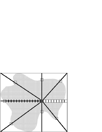
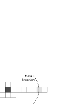
Figure 1: Basic schema of the segmentation procedure.

1.2 Feature extraction

Once the masses have been segmented out of the surrounding normal tissue, a set of suitable features are computed in order to allow a decision-making system to distinguish benign from malignant lesions [13, 14, 15, 16]. The degree of malignancy of a lesion is generally correlated to the appearance of arms and spiculations on the mass boundary. The more irregular the mass shape, the higher the degree of malignancy possibly associated to that lesion. Our CADi system extracts 16 features from the segmented lesions: the mass area $A$; the mass perimeter $P$; the circularity $C={4\pi A}/{P^{2}}$; the mean and the standard deviation of the normalized radial length (i.e. the Euclidean distance from the center of mass of the segmented lesion to the $i^{\rm th}$ pixel on the perimeter and normalized to the maximum distance for that mass); the radial length entropy (i.e. a probabilistic measure computed from the histogram of the normalized radial length as $E=-\sum_{k=1}^{N_{\rm bins}}P_{k}\log{P_{k}}$, where $P_{k}$ is the probability that the normalized radial length is between $d(i)$ and $d(i)+1/N_{\rm bins}$ and $N_{\rm bins}$ is the number of bins the normalized histogram has been divided in); the zero crossing (i.e. a count of the number of times the radial distance plot crosses the average radial distance); the maximum and the minimum axis of the lesion; the mean and the standard deviation of the variation ratio (i.e. the modulus of the variations of the radial lengths from their mean value are computed and only those exceeding the value $var_{\rm max}/2$, where $var_{\rm max}$ is the maximum variation, are considered as dominant variations and averaged); the convexity (i.e. the ratio between the mass area and the area of the smallest convex containing the mass); the mean, the standard deviation, the skewness and the kurtosis of the mass grey-level intensity values.

The 16 features were chosen with the aim of enlightening the spiculation characteristics of the lesions. The first 12 features in the above description are related to the mass shape and have some evident correlations with the degree of spiculation of the lesions. Nevertheless, the remaining 4 features derived from the grey-level intensity distribution of the segmented area also aim at investigating the degree of mass spiculation: the standard deviation, the skewness and the kurtosis carry out the information about irregularities characterizing the mass, whereas the mean value accounts for an offset to be referred to these three parameters.

1.3 Classification

The $16$ features extracted from each lesion are classified by a standard three-layer feed-forward neural network with $n$ input, $h$ hidden and two output neurons. A supervised training based on the back-propagation algorithm with sigmoid activation functions both for the hidden and the output layer has been performed. The performances of the training algorithm were evaluated according to the 5$\times$2 cross validation method [17]. It is the recommended test to be performed on algorithms that can be executed 10 times because it can provide a reliable estimate of the variation of the algorithm performances due to the choice of the training set. This method consists in performing 5 replications of the 2-fold cross validation method [18]. At each replication, the available data are randomly partitioned into 2 sets ($A_{i}$ and $B_{i}$ for $i=1,\dots 5$) with an almost equal number of entries. The learning algorithm is trained on each set and tested on the other one. The system performances are given in terms of the sensitivity and specificity values, where the sensitivity is defined as the true positive fraction (fraction of malignant masses correctly classified by the system), whereas the specificity as the true negative fraction (fraction of benign masses correctly classified by the system). In order to show the trade off between the sensitivity and the specificity, a Receiver Operating Characteristic (ROC) analysis has been performed [19, 20]. The ROC curve is obtained by plotting the true positive fraction versus the false positive fraction of the cases (1 - specificity), computed while the decision threshold of the classifier is varied. Each decision threshold results in a corresponding operating point on the curve.

2 Image dataset

The image dataset used for this study has been extracted from the database of mammograms collected in the framework of a collaboration between physicists from several Italian Universities and INFN (Istituto Nazionale di Fisica Nucleare) Sections, and radiologists from several Italian Hospitals [21, 22]. The mammograms come both from screening and from the routine work carried out in the participating Hospitals. The $18\times 24$ cm² mammographic films were digitized by a CCD linear scanner (Linotype Hell, Saphir X-ray), obtaining images characterized by a $85\mu$m pixel pitch and a 12-bit resolution. The pathological images are fully characterized by a consistent description, including the radiological diagnosis, the histological data and the coordinates of the center and the approximate radius (in pixel units) of a circle drawn by the radiologists around the lesion (truth circle). Mammograms with no sign of pathology are stored as normal images only after a follow up of at least three years.

A set of 226 massive lesions were used in this study: 109 malignant and 117 benign masses were extracted from single-view cranio-caudal or lateral mammograms. The dataset we analyzed can be considered as representative of the patient population that is sent for biopsy under the current clinical criteria.

3 Results

The 226 massive lesions were segmented by the system and shown to an experienced radiologist, whose assistance in accepting or rejecting the proposed mass contours was essential for the evaluation of the segmentation algorithm efficiency. Despite the borders of the massive lesions are usually not very sharp in mammographic images, the segmentation procedure we carried out leads to a quite accurate identification of the mass shapes, as can be noticed in fig. 2.

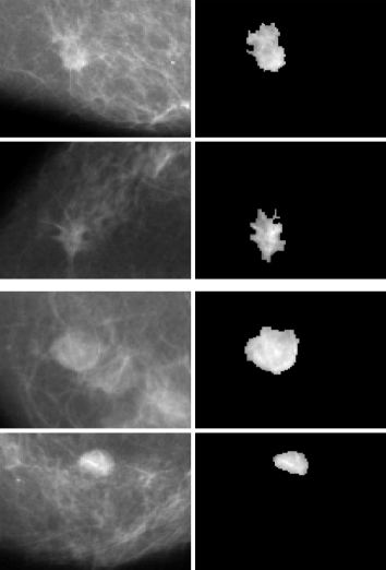
Figure 2: Examples of segmented masses: two malignant masses (top) and two benign masses (bottom).

The radiologist confirmed only the segmented masses whose contour was sufficiently close to that she would have drawn by hand on the image. The dataset of 226 cases available for our analysis was reduced to 200 successfully-segmented masses (95 malignant and 105 benign masses), thus corresponding to an efficiency $\epsilon=88.5\%$ for the segmentation algorithm.

Once the 16 features were extracted from each well-segmented mass, 5 different train and 5 different test sets for the 5$\times$2 cross validation analysis were prepared by randomly assigning each of the 200 vectors of features to the train or test set for each of the 5 different trials. The optimization of the network performances was obtained in our case by assigning 3 neurons to the hidden layer, resulting in a final architecture for the net of 16 input, 3 hidden and 2 output neurons.

The sensitivity and specificity our learning algorithm realized on each dataset are shown in tab. 1.

Table 1: Evaluation of the performances of the standard back-propagation learning algorithm for the neural classifier according to the 5$\times$2 cross validation method.

Train Set	Test Set	Sens. (%)	Spec. (%)
$A_{1}$	$B_{1}$	78.7	84.9
$B_{1}$	$A_{1}$	77.1	84.6
$A_{2}$	$B_{2}$	78.7	79.3
$B_{2}$	$A_{2}$	77.1	78.9
$A_{3}$	$B_{3}$	80.9	72.9
$B_{3}$	$A_{3}$	77.1	78.7
$A_{4}$	$B_{4}$	79.2	77.4
$B_{4}$	$A_{4}$	78.7	78.9
$A_{5}$	$B_{5}$	75.6	81.8
$B_{5}$	$A_{5}$	78.0	74.0

As can be noticed, the performances the neural classifier achieves are robust, i.e. almost independent of the partitioning of the available data into the train and test sets. The average performances achieved in the testing phase are 78.1% for the sensitivity and 79.1% for the specificity. The ROC curve obtained in the classification of the test set $B_{2}$, containing 100 patterns derived from 47 malignant masses and 53 benign masses, is reported in fig. 3. To this curve belongs the operating point whose values of sensitivity (78.7%) and specificity (79.3%) are closer to the average values achieved on the test sets by the ten different neural networks, as shown in tab. 1. As the classifier performances are conveniently evaluated in terms of the area $A_{z}$ under the ROC curve, we have estimated this parameter for the curve plotted in fig. 3, obtaining $A_{z}=0.80\pm 0.04$, where the standard error has been evaluated according to the formula given by Hanley and McNeil [20].

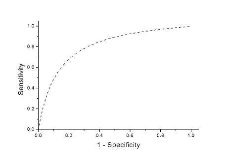
Figure 3: ROC curve obtained in the classification of the test set $B_{2}$ (see tab. 1).

4 Conclusions and discussion

The system for the classification of mammographic massive lesions into malignant and benign we realized aims at improving the radiologist’s visual diagnosis of the degree of the lesion malignancy. The system is a semi-automated one, i.e. it segments and analyzes lesions from physician-located rectangular ROIs. As mass segmentation plays a key role in such kind of systems, most efforts have been devoted to the realization of a robust segmentation technique. It is based on edge detection and it works with a comparable efficiency both on malignant and benign masses. The segmentation efficiency $\epsilon=88.5\%$ has been evaluated with the assistance of an experienced radiologist who accepted or rejected each segmented mass. With respect to a number of automated or semi-automated systems with a similar purpose and using a similar approach already discussed in the literature [8, 9, 10, 11], the system we present is characterized by a robust segmentation technique: it is based on an edge-detection algorithm completely free from any application-dependent parameter.

Sixteen features based on shape, size and intensity have been extracted out of each segmented area and merged by a neural decision-making system. The neural network performances have been evaluated in terms of the ROC analysis, obtaining an estimated area under the ROC curve $A_{z}=0.80\pm 0.04$. It gives the indication that the segmentation procedure we developed provides a quite accurate approximation of the mass shapes and that the features we took into account for the classification have a good discriminating power.

References

- [1] R.T. Greenlee, M.B. Hill-Harmon, T. Murray, M. Thun, Ca-Cancer J. Clin. 51(1) (2001) 15. Err. in: Ca-Cancer J. Clin. 51(2) (2001) 144.
- [2] F. Levi, F. Lucchini, E. Negri, P. Boyle, C. La Vecchia, Ann. Oncol. 14 (2003) 490.
- [3] H.C. Zuckerman, Breast cancer: diagnosis and treatment, pp 152–72. I.M. Ariel and J.B. Cleary eds, New York: McGraw-Hill, 1987.
- [4] D.D. Adler and M.A. Helvie, Curr. Opin. Radiol. 4(5) (1992) 123.
- [5] Z. Huo, M.L. Giger, C.J. Vyborny, D.E. Wolverton, R.A. Schmidt, K. Doi, Acad. Radiol. 5(3) (1998) 155.
- [6] Z. Huo, M.L. Giger, C.J. Vyborny, D.E. Wolverton, C.E. Metz, Acad. Radiol. 7(12) (2000) 1077.
- [7] B. Sahiner, H.P. Chan, N. Petrick, M.A. Helvie, M.M. Goodsitt, Med. Phys. 25(4) (1998) 516.
- [8] M.A. Wirth and A. Stapinski, Proc. SPIE 5150 (2003) 1995.
- [9] A. Amini, S. Tehrani, T. Weymouth, Proc. Second Int. Conf. Computer Vision, Tarpon Springs, FL (1988) 95.
- [10] B. Sahiner, N. Petrick, H.P. Chan, L.M. Hadjiiski, C. Paramagul, M.A. Helvie, M.N. Gurcan, IEEE Trans. Med. Im. 20(12) (2001) 1275.
- [11] M.A. Kupinski and M.L. Giger, IEEE Trans. Med. Im. 17(4) (1998) 510.
- [12] D.R. Chen, R.F. Chang, W.P. Kuo, M.C. Chen, Y.L. Huang, Ultrasound Med. Biol. 28(10) (2002) 1301.
- [13] I. Christoyianni, A. Koutras, E. Dermatas, G. Kokkinakis, Proc. IEEE ICECS 1 (1999) 117.
- [14] W. Qian, L. Li, L.P. Clarke, Med. Phys. 26 (1999) 402.
- [15] L. Hadjiiski, B. Sahiner, H.P. Chan, N. Petrick, M.A. Helvie, M. Gurcan, Med. Phys. 28(11) (2001) 2309.
- [16] B. Sahiner, H.P. Chan, N. Petrick, M.A. Helvie, L.M. Hadjiiski, Med. Phys. 28(7) (2001) 1455.
- [17] T.G. Dietterich, Neural Computation 10(7) (1998) 1895.
- [18] M. Stone, J. Royal Statistical Soc. B 36 (1974) 111.
- [19] C.E. Metz, Invest. Radiol. 21(9) (1986) 720.
- [20] J.A. Hanley and B.J. McNeil, Radiology 143(1) (1982) 29.
- [21] U. Bottigli, et al., Proc. SPIE 4684 (2002) 1301.
- [22] R. Bellotti, et al., Proc. IEEE Nucl. Science Symp. (2004) N33-173.