Coarse-grained analysis of a lattice Boltzmann model for planar streamer fronts

Abstract

We study the traveling wave solutions of a lattice Boltzmann model for the planar streamer fronts that appear in the transport of electrons through a gas in a strong electrical field. To mimic the physical properties of the impact ionization reaction, we introduce a reaction matrix containing reaction rates that depend on the electron velocities. Via a Chapman–Enskog expansion, one is able to find only a rough approximation for a macroscopic evolution law that describes the traveling wave solution. We propose to compute these solutions with the help of a coarse-grained time-stepper, which is an effective evolution law for the macroscopic fields that only uses appropriately initialized simulations of the lattice Boltzmann model over short time intervals. The traveling wave solution is found as a fixed point of the sequential application of the coarse-grained time-stepper and a shift-back operator. The fixed point is then computed with a Newton-Krylov Solver. We compare the resulting solutions with those of the approximate PDE model, and propose a method to find the minimal physical wave speed.

March 3, 2024

I Introduction

When a gas of neutral atoms or molecules is exposed to a strong electrical field, a small initial seed of electrons can lead to an ionization avalanche. Indeed, the seed electrons are accelerated by the field and gain enough energy to ionize the neutral atoms when they collide. The two slow electrons that emerge from this reaction, i.e. the impact and the ionized electron, are again accelerated by the field and cause, on their turn, an ionization reaction. Simultaneously the electrical field is locally modified because of the charge creation. This interplay between the dynamics of the electrons and the electrical field can lead to a multitude of phenomena studied in plasma physics such as arcs, glows, sparks and streamers.

In this article we will focus on the initial field driven ionization that can lead to traveling waves known as streamer fronts. These waves have previously been studied by Ebert et al. ebert who introduced and analyzed the minimal streamer model, a one-dimensional model for the propagation of planar streamer fronts. This model consists of two coupled non-linear PDEs: a reaction-convection-diffusion equation for the evolution of the electron density and a Poisson-like evolution equation for the electrical field. The reaction term is based on the Townsend approximation that expresses the growth of the number of electrons as a function of the local electrical field.

During the last two decades, however, a lot of progress has been made in the microscopic understanding of impact ionization reactions in atomic and molecular systems. In this reaction an impact electron ionizes the target and kicks out an additional electron. There are several successful theories that can predict the exact probability distribution of the escaping electron bray ; malegat ; pindzola ; rescigno . In the next decade, we expect that the theoretical tools will be able to accurately predict the microscopic physics of electron impact on molecular targets such as N₂ and O₂, the most important molecules in the composition of air. This progress in the understanding of the impact ionization reaction, however, has not been incorporated in the description of the macroscopic behavior such as the minimal streamer front of Ebert et al. Instead, such models still make use of a phenomenological approximation to the reactions, such as the Townsend approximation. This article extends the minimal streamer model and incorporates more microscopic information. We model the system by a Boltzmann equation, which is constructed such that the cross sections in the collision integral resemble the true microscopic cross sections.

To find the traveling wave solutions of this more microscopic model, we exploit a separation of time scales between the relaxation of the electron distribution function to a local equilibrium and the evolution of the macroscopic fields (electron density and electrical field). It is known from kinetic theory that the first process is fast: once initialized, it takes a molecular gas not more than a few collisions to relax to its equilibrium state.

In kinetic theory, the fast times scales are often eliminated from the problem by assuming a local equilibrium distribution function which leads to a reaction-diffusion model with transport coefficients that depend on the local electrical field. This reduction method, however, is only successful in the absence of steep gradients in the electron density uhlenbeck , an assumption not valid for the planar streamer fronts that have, typically, very steep increases in the electron density.

In this article, we take an alternative route and find the traveling wave solution through a so-called coarse-grained time-stepper (CGTS) that exploits the separation of time scales to extract the effective macroscopic behavior. This method was proposed by Kevrekidis et al. manifesto and the numerical aspects of its application to find traveling wave solutions of lattice Boltzmann models have recently been studied samaey . The time-stepper uses a sequence of computational steps to evolve the macroscopic state. This sequence involves: (1) a lifting step, which creates an appropriate electron distribution function for a given electron density, (2) a simulation step, where the lattice Boltzmann model is evolved over a coarse-grained time step $\Delta T$, and (3) a restriction step, where the macroscopic state is extracted from the electron distribution function. This method does not derive effective equations explicitly, and therefore allows steep gradients to be present. We compare our results with those obtained by deriving an approximate macroscopic PDE model through the more traditional Chapman-Enskog expansion. The paper therefore illustrates the applicability of the coarse-grained time-stepper on a non-trivial problem where the exact macroscopic equations are hard to derive.

The outline of the paper is as follows. In section II, we shortly review the physics of the impact ionization reaction and the streamer fronts, and recapitulate the Boltzmann equations. In section III, we derive from the Boltzmann equation a lattice Boltzmann model with multiple velocities and discuss how the ionization reaction, external field and electron diffusion are incorporated in the model. Section IV derives a macroscopic PDE from the model using the Chapman-Enskog expansion and discusses the minimal velocity of the traveling waves. Section V formulates the coarse-grained time-stepper and VI how the traveling wave solutions are found. Finally in section VII, we have some numerical results.

II Model

II.1 The physics of the impact ionization reaction

The impact ionization reaction is a microscopic reaction where electrons with, typically, an energy around 50eV collide with an atom or a molecule and ionize this target. The reaction rates of this process depend sensitively on a number of parameters. Let us consider the simplest system: an electron hits a hydrogen atom with a bound electron in its ground state. When the incoming electron has an energy larger than the binding energy of the electron in the atom, it can kick out, with a certain probability, the bound electron that will escape, together with the impact electron, from the atom. The total energy of the two electrons after the collision is equal to the energy of the incoming electron minus the original binding energy of the bound electron.

The reaction rates of this process are expressed by cross sections; these are probabilities that a certain event will take place. One such cross section is the triple differential cross section, which is the probability to find after the collision one electron escaping in the direction $(\theta_{1},\phi_{1})$ with an energy $E_{1}$ and a second electron escaping in the direction $(\theta_{2},\phi_{2})$ with an energy $E_{2}$, where the angles are measured with respect to the axis defined by the momentum of the incoming electron. Since the two electrons repel each other, it is more likely that they escape in opposite directions wannier .

Figure 1: A sketch of the typical shape of the impact ionization cross section ( see the experimental results in hu ). On top, we show the total cross section as a function of the impact energy where below a threshold energy of 25eV no reactions take place. In the proposed model we distinguish between slow particles with an energy below this threshold that do not react and fast particles with their energy above this threshold. The fast reacting particles experience a cross section of $R$, as indicated by the dashed line. In the bottom figure, we show the energy differential cross section for the escaping electron, where the total energy of the escaping electrons is 25eV. Since the two electrons are indistinguishable there is a symmetry. In our five speed model, we make the approximation that the two electrons can only escape with equal energy sharing.

When this cross section is integrated over all angles $(\theta_{1},\phi_{1})$ and $(\theta_{2},\phi_{2})$ of the escaping electrons and all possible ratios of $E_{1}/E_{2}$ of the electron energies, we get the total cross section. This is the total probability that the incoming electron will cause an ionization event. This total cross section depends on the energy of the incoming electron and is zero when the energy of the incoming electron is below the binding energy of the bound electron. Just above this binding energy, there is a steep rise in the cross section that is known as a threshold. Just above this threshold the cross section is the largest and as we further increase the energy the cross section diminishes. This is illustrated in figure 1 (top).

When the cross section is integrated of the angles only, but not over the relative energies, we get the so called energy differential cross section, which is the probability of causing an ionization event with a given relative energy of the two electrons. In contrast with the electron directions, there is no pronounced preference for the energy sharing between the two electrons, see figure 1 (bottom). It is only slightly more likely that two electrons will come out with unequal energy.

Recently, several theoretical methods have successfully predicted the directions of the escaping electrons, the total cross section and the energy differential cross section in the hydrogen atom. We name exterior complex scaling rescigno , time dependent close coupling pindzola , HRW-SOW malegat and convergent close coupling bray .

When the electron hits a molecular system instead of an atom, the physics is complicated by the extra degrees of freedom. The cross sections now depend on both the orientation and internuclear coordinates of the molecule at the moment of electron impact, as is seen in processes where two electrons are ejected from molecules after it is hit by a photon vanroose ; weber . Therefore, there will be some random terms in the reaction cross section, which will need to be included in a realistic microscopic model. In this paper, we will model the microscopic interactions using a Boltzmann equation, which is still deterministic; extensions that accurately account for random effects will be treated in future work. However, we note that the coarse-grained time-stepper approach that is used in this work has already been applied successfully to study systems with stochastic effects qiao .

II.2 Review of the physics of streamer fronts.

Ebert et al. ebert introduced the minimal streamer model. It consists of two coupled non-linear PDEs: a reaction-convection-diffusion equation for the evolution of the electron density and an equation that relates the change in the electrical field to the charge flux. The electron density evolves because of the drift due to the electrical field, the electron diffusion and the ionization reaction, which is formulated in the Townsend approximation. The reaction rate is then given by an exponential that depends on the strength of the local electrical field. The evolution of the electrical field is determined by Poisson’s law of electrostatics where the field changes because of the charge creation by the ionization reaction. This minimal streamer model exhibits both negatively and positively charged fronts. The first moves in the direction of the electrical field, while the positively charged moves in the opposite direction and can only propagate because of the electron diffusion and the ionization reactions. Each of these fronts appears as a one-parameter family of uniformly translating solutions (since any translate of the wave is also a solution).

In our extension of the Ebert model, we replace the reaction-diffusion equation for the evolution of the electron density with a Boltzmann equation for the one-electron distribution function $f(\mathbf{x},\mathbf{v},t)$, that counts the number of electrons in the phase-space volume element bounded by position $\mathbf{x}$ and $\mathbf{x+dx}$ and by speed $\mathbf{v}$ and $\mathbf{v+dv}$. The Boltzmann equation is

$$\frac{\partial f(\mathbf{x},\mathbf{v},t)}{\partial t}+\mathbf{v}\cdot\frac{\partial f(\mathbf{x},\mathbf{v},t)}{\partial x}+\mathbf{E}(\mathbf{x},t)\cdot\frac{\partial f(\mathbf{x},\mathbf{v},t)}{\partial v}=\Omega(\mathbf{x},t),$$ (1)

where $\mathbf{E}(\mathbf{x},t)$ is the external electrical field and $\Omega(\mathbf{x},t)$ is the collision operator, an integral operator that integrates the cross sections of the ionization reaction over the velocity space. This Boltzmann equation is coupled to an evolution equation for the electrical field. Because additional electrons are created, the local charge density changes the electrical field through the Poisson law

$$\bnabla\cdot{\mathbf{E}}(\mathbf{x},t)=q(\mathbf{x},t),$$

where $q(x,t)=(n_{+}-n_{e})e/q_{0}$ is the charge distribution. Here, $n_{+}$ represents the number of ions, $n_{e}$ is the number of electrons and $q_{0}$ a unit of charge.

We now connect the change in electrical field with the change in the charge distribution. We have

$$\frac{\partial q(\mathbf{x},t)}{\partial t}+\bnabla\cdot{\mathbf{j}}(\mathbf{x},t)=0$$

in which $\mathbf{j}(\mathbf{x},t)$ is the charge flux. This leads to an equation for the evolution of the electrical field,

$$\frac{\partial\mathbf{E}(\mathbf{x},t)}{\partial t}+\mathbf{j}(\mathbf{x},t)=0.$$ (2)

Since we assume that the ions are immobile, the flux $\mathbf{j}(\mathbf{x},t)$ is solely determined by the one-particle distribution function $f(\mathbf{x},\mathbf{v},t)$ of the electrons.

Our extension of the minimal streamer model is now the coupled evolution of eq. (1) and (2). Note that the set of coupled equations is very similar to the Wigner-Poisson problem wigner used to model electron transport through diodes.

III Lattice Boltzmann Discretization

Together with the impact ionization cross sections, the coupled equations (1) and (2) are a non-linear integro-differential equation coupled to a scalar partial differential equation for the electrical field. This equation in its full dimension is hard to solve, both analytically and numerically. As a first step, we look at the one-dimensional streamer fronts of the Boltzmann equation in the lattice Boltzmann discretization.

III.1 Discretization of the Boltzmann equation

In this section, we discretize the one-dimensional Boltzmann equation (1). The distribution functions $f(x,v,t)$ are discretized on a lattice in space, velocity and time. The grid spacing is $\Delta x$ in space and $\Delta t$ in time. The velocity grid of $v_{i}$ is chosen such that the distance traveled in a single time step, $v_{i}\Delta t$, is a multiple of the grid distance $\Delta x$, or in short

$$v_{i}=i\frac{\Delta x}{\Delta t},\hskip 28.45274pt\mbox{with}\hskip 28.45274pti\in{\mathcal{S}}.$$

Typically, only a small set of discrete velocities is used. A discretization with three grid points on the velocity grid has a set $\mathcal{S}=\{-1,0,1\}$ and is called a D1Q3 model. A discretization with five grid points has $\mathcal{S}=\{-2,-1,0,1,2\}$ and is a D1Q5 model. The size of the set $\mathcal{S}$ is denoted by $m$. We will also denote $c_{i}=v_{i}\Delta t/\Delta x$ for the dimensionless velocity.

Note that, for ease of notation, we will also use the set $\mathcal{S}$ to index matrices. For example, the result of a linear operator $A$ working on a vector $v_{j\in\mathcal{S}}$ will be denoted as $\sum_{i\in\mathcal{S}}A_{ij}v_{j}$, where both the indices $i$ and $j$ are in $\mathcal{S}$. The means that the $A_{-2,-2}$ matrix element with $\mathcal{S}=\{-2,-1,0,1,2\}$ is the matrix element in the upper left corner of the matrix.

We start from the continuous equation for the distribution function in the discrete point $(x+v_{i}\Delta t,v_{i})$ in phase space at time $t$. In the absence of external forces, the Boltzmann equation in this point reads

$$\frac{\partial f(x+v_{i}\Delta t,v_{i},t)}{\partial t}+v_{i}\frac{\partial f(x+v_{i}\Delta t,v_{i},t)}{\partial x}$$

$$=\Omega(x+v_{i}\Delta t,v_{i},t)$$ (3)

A discrete lattice Boltzmann equation is now obtained by replacing the time derivative with an explicit forward difference, the introduction of an upwind discretization of the convection term and a downwind discretization of the collision term $\Omega(x+v_{i}\Delta t,v_{i},t)$ and replace it with $\Omega(x,v_{i},t)$ cao ,

$$\frac{f(x+v_{i}\Delta t,v_{i},t+\Delta t)-f(x+v_{i}\Delta t,v_{i},t)}{\Delta t}$$

$$+v_{i}\frac{f(x+v_{i}\Delta t,v_{i},t)-f(x,v_{i},t)}{v_{i}\Delta t}=\Omega(x,v_{i},t).$$ (4)

Note that this discretization of the spatial derivative becomes less accurate for the largest speeds in the set $\mathcal{S}$. Indeed, in the five speed model, for example, the largest speed is $v_{\pm 2}=\pm 2\Delta x/\Delta t$, and the convection term will be calculated from the difference between $f(x+v_{\pm 2}\Delta t,v_{\pm 2},t)$ and $f(x,v_{\pm 2},t)$, which is $2\Delta x$ apart. The discretization error is then proportional to $2\Delta x$.

Equation (4) reduces to

$$f_{i}(x+v_{i}\Delta t,t+\Delta t)-f_{i}(x,t)=\Delta t\,\Omega_{i}(x,t),$$ (5)

where we have introduced the shorthand $f_{i}(x,t)$ for $f(x,v_{i},t)$ and $\Omega_{i}(x,t)$ for $\Omega(x,v_{i},t)$ with $i\in\mathcal{S}$.

III.2 The collision term

The collision term consists out of two parts

$$\Delta t\Omega_{i}=\Omega_{i}^{\mbox{\scriptsize diff}}+\Omega_{i}^{\mbox{\scriptsize reaction}}$$ (6)

where the first term will model the electron diffusion, the second term the ionization reactions and the third term the influence of the external force. Note that we also incorporated $\Delta t$ in the notation. We will now discuss the two terms individually.

The first term models the electron diffusion as a BGK relaxation process BGK . In this approximation, it assumed that the distribution is attracted to a local equilibrium distribution function $f_{i}^{eq}$,

$$\Omega_{i}^{\mbox{\scriptsize diff}}=-\frac{1}{\tau}\left(f_{i}-f_{i}^{eq}\right),$$ (7)

with $f_{i}^{eq}(x,t)$ the equilibrium distribution for electron diffusion. In the five speed model, we choose

$$f_{i}^{eq}=w_{i}^{eq}\rho\quad\mbox{with}\quad w_{i}^{eq}=\left\{0,1/4,2/4,1/4,0\right\}$$ (8)

and $\rho(x,t)$ the electron density. This choice of equilibrium weights conserves the number of electrons, but does not conserve momentum as a traditional fluid would do. Indeed, the electrons diffuse because they randomly change their direction during the elastic collisions with the much heavier neutral molecular particles. We further chose the weights such that there are no fast particles under diffusive equilibrium. The relaxation time $\tau$ is related to the electron diffusion coefficient

$$\tau=\frac{1}{2}+\frac{D}{\sum_{i\in\mathcal{S}}c_{i}^{2}w_{i}^{eq}}\frac{\Delta t}{\Delta x^{2}}.$$ (9)

Note that, in the literature, the relaxation time $\tau$ is often characterized by its inverse $\omega=1/\tau$.

The second term in (6) is the reaction term $\Omega_{i}^{\mbox{\scriptsize reaction}}$ that is modelled with a $m\times m$ matrix $\mathcal{R}$

$$\Omega_{i}^{\mbox{\scriptsize reaction}}=\Delta t\sum_{j\in\mathcal{S}}\mathcal{R}_{ij}f_{j},$$ (10)

which represents the velocity dependent reaction rates and allows us to select between slow and fast particles.

For the five speed model, we choose a reaction matrix

$$\mathcal{R}=\left(\begin{array}[]{ccccc}-R&0&0&0&0\\ R&0&0&0&R\\ 0&0&0&0&0\\ R&0&0&0&R\\ 0&0&0&0&-R\end{array}\right)$$ (11)

that describes how the reaction cross sections depend on the velocities of the particles. Each time step $\Delta t$, a fraction $R$ of the particles with speed $v_{\pm 2}$ will collide and cause a ionization reaction. The reaction rate $R$ is chosen to match the height of the cross section, see figure 1. Since the colliding fast particles transfer their energy to the bound electron, they will loose energy. Therefore, the number of particles with speed $v_{\pm 2}$ diminishes with a rate $-R\Delta t$ and we have $\mathcal{R}_{-2,-2}=\mathcal{R}_{+2,+2}=-R$. At the same time, the number of slow electrons increases because both the impact electron and the ionization electron emerge as slow particles with speed $v_{\pm 1}$. Because of the Coulomb repulsion, the two slow electrons are more likely to emerge in opposite directions and we choose the rates such that one electron emerges with speed of $v_{-1}$ and the other with $v_{+1}$.

This choice of model parameters ensures that the energy balance during the ionization reaction is not violated. As discussed in section II.1, the energy of the incoming electron is larger that the sum of the energies of the escaping electrons because some of the impact energy covers the binding energy of the bound electron. In the above model, a single ionization reaction transforms one electron with speed $v_{+2}$ into two electrons with, respectively, speed $v_{+1}$ and speed $v_{-1}$. The energy of the impact electron is $mv_{+2}^{2}/2=2m\Delta x/\Delta t$, while the sum of the escaping electrons is merely $2mv_{1}^{2}/2=m\Delta x/\Delta t$, where $m$ is the mass of the electron. So a portion $m\Delta x/\Delta t$ of the impact energy covers the binding energy. For our model, this is half of the initial impact energy; for more general problems other values are possible.

III.3 External Force

We now derive a discretization of the $E\frac{\partial f_{i}}{\partial v}$ term that models the external force in the Boltzmann equation. We start by expanding

$$\frac{\partial\mathbf{f}}{\partial v}=a_{0}\mathbf{v}_{0}+a_{1}\mathbf{v}_{1}+\ldots+a_{m-1}\mathbf{v}_{m-1},$$

where $\mathcal{V}=\{\mathbf{v}_{0},\mathbf{v}_{1},\ldots,\mathbf{v}_{m-1}\}$ forms a linear independent set of vectors in $\mathbb{R}^{m}$. We find the coefficients $a_{0},a_{1},\ldots,a_{m-1}$ by enforcing the Galerkin condition.

$$\left(\frac{\partial\mathbf{f}}{\partial v}-\sum_{i=0}^{m-1}a_{i}\mathbf{v}_{i}\right)\perp\mathcal{V}$$

In the current paper, we choose a particular set of vectors in $\mathcal{V}$, namely the polynomials $\{1,v,v^{2},\ldots,v^{m-1}\}$ discretized in the points $v_{i}$. For the five speed example the vectors are, besides their powers of $\Delta x/\Delta t$,

$$\mathcal{V}=\left\{\left(\begin{array}[]{c}1\\ 1\\ 1\\ 1\\ 1\end{array}\right),\left(\begin{array}[]{c}-2\\ -1\\ 0\\ 1\\ 2\end{array}\right),\left(\begin{array}[]{c}4\\ 1\\ 0\\ 1\\ 4\end{array}\right),\left(\begin{array}[]{c}-8\\ -1\\ 0\\ 1\\ 8\end{array}\right),\left(\begin{array}[]{c}16\\ 1\\ 0\\ 1\\ 16\end{array}\right)\right\}$$

The Galerkin condition leads to the linear system

$$\left(\begin{array}[]{ccccc}m&0&\alpha&0&\beta\\ 0&\alpha&0&\beta&0\\ \alpha&0&\beta&0&\gamma\\ 0&\beta&0&\gamma&0\\ \beta&0&\gamma&0&\delta\end{array}\right)\left(\begin{array}[]{c}a_{0}\\ a_{1}\\ a_{2}\\ a_{3}\\ a_{4}\end{array}\right)=\left(\begin{array}[]{c}\mathbf{v}_{0}^{t}\cdot\frac{\partial\mathbf{f}}{\partial v}\\ \mathbf{v}_{1}^{t}\cdot\frac{\partial\mathbf{f}}{\partial v}\\ \mathbf{v}_{2}^{t}\cdot\frac{\partial\mathbf{f}}{\partial v}\\ \mathbf{v}_{3}^{t}\cdot\frac{\partial\mathbf{f}}{\partial v}\\ \mathbf{v}_{4}^{t}\cdot\frac{\partial\mathbf{f}}{\partial v}\end{array}\right)$$ (12)

where $\alpha=\sum_{i\in\mathcal{S}}v_{i}^{2}$,$\beta=\sum_{i\in\mathcal{S}}v_{i}^{4}$, $\gamma=\sum_{i\in\mathcal{S}}v_{i}^{6}$ and $\delta=\sum_{i\in\mathcal{S}}v_{i}^{8}$.

To calculate the right-hand side of (12) we make a detour around the continuous representation. We note that

$$\mathbf{v}_{l}^{t}\cdot\frac{\partial\mathbf{f}}{\partial v}=\int_{-\infty}^{+\infty}v^{l}\frac{\partial f(x,v,t)}{\partial v}dv,$$ (13)

where $l\in\{0,1,\ldots,m-1\}$. Because of our particular choice of basis vectors and the fact that there are no particles with infinite velocities, we have that

$$\int_{-\infty}^{+\infty}v^{l}\frac{\partial f(x,v,t)}{\partial v}dv +\int_{-\infty}^{+\infty}f(x,v,t)\frac{\partial v^{l}}{\partial v}dv$$ (14)

$$=v^{l}f(x,v,t)|_{-\infty}^{+\infty}=0$$

or, in other words,

$$\mathbf{v}_{l}^{t}\cdot\frac{\partial\mathbf{f}}{\partial v} = -i\int_{-\infty}^{+\infty}f(x,v,t)v^{l-1}dv$$ (15)

$$= -l\sum_{j\in\mathcal{S}}v_{j}^{l-1}f_{j}$$

With the help of

$$N=\left(\begin{array}[]{ccccc}0&0&0&0&0\\ -1&-1&-1&-1&-1\\ -2v_{-2}&-2v_{-1}&-2v_{0}&-2v_{1}&-2v_{2}\\ -3{v_{-2}}^{2}&-3{v_{-1}}^{2}&-3{v_{0}}^{2}&-3v_{{1}}^{2}&-3{v_{2}}^{2}\\ -4{v_{-2}}^{3}&-4{v_{-1}}^{3}&-4{v_{0}}^{3}&-4v_{{1}}^{3}&-4{v_{2}}^{3}\end{array}\right),$$ (16)

we can now define

$$V\!\!=\!\!\!\left(\begin{array}[]{ccccc}1&v_{-2}&{v_{-2}}^{2}&{v_{-2}}^{3}&{v_{-2}}^{4}\\ 1&v_{-1}&{v_{-1}}^{2}&{v_{-1}}^{3}&{v_{-1}}^{4}\\ 1&v_{0}&{v_{0}}^{2}&{v_{0}}^{3}&{v_{0}}^{4}\\ 1&v_{1}&{v_{1}}^{2}&{v_{1}}^{3}&{v_{1}}^{4}\\ 1&v_{2}&{v_{2}}^{2}&{v_{2}}^{3}&{v_{2}}^{4}\end{array}\right)\!\left(\begin{array}[]{ccccc}m&0&\alpha&0&\beta\\ 0&\alpha&0&\beta&0\\ \alpha&0&\beta&0&\gamma\\ 0&\beta&0&\gamma&0\\ \beta&0&\gamma&0&\delta\end{array}\right)^{-1}\!\!\!\!\!N,$$ (17)

and calculate the external force term as

$$E(x,t)\frac{\partial f_{i}(x,t)}{\partial v}=E(x,t)\sum_{j\in\mathcal{S}}V_{ij}f_{j}(x,t),$$ (18)

where the elements of $\mathcal{S}$ denote matrix elements.

From eq. (18), it is clear that we can include the external force as an additional collision term in the right-hand side of the lattice Boltzmann equation.

III.4 Flux

The evolution of the electrical field $E(x,t)$ is determined by the net flux $j(x,t)$ of electrons as expressed in (2). We discretize (2) on a staggered grid with grid points halfway between the grid points of the lattice Boltzmann model. The flux is defined as the number of particles that move between grid points (pass through an interface) within a single time step. For the five speed model, we have

$$j(x+\Delta x/2, t) =f_{1}(x+\Delta x,t)-f_{-1}(x,t)$$

$$+f_{2}(x+\Delta x,t)-f_{-2}(x,t)$$

$$+f_{2}(x+2\Delta x,t)-f_{-2}(x-\Delta x,t)$$

III.5 Coupled equations

The coupled equations (1) and (2) for the evolution of the electron distribution functions and the electrical field is now, after discretization,

$$f_{i}(x+v_{i}\Delta t,t+\Delta t)-f_{i}(x,t)=\\ -\frac{1}{\tau}\big{(}f_{i}(x,t)-f_{i}^{eq}(x,t)\big{)}+\sum_{j\in\mathcal{S}}\Delta t\mathcal{R}_{ij}f_{j}(x,t)\\ -\frac{\left(E(x-\Delta x/2,t)+E(x+\Delta x/2,t)\right)}{2}\sum_{j\in\mathcal{S}}{\Delta tV_{ij}f_{j}(x,t)}$$ (20)

$$E(x+\frac{\Delta x}{2},t+\Delta t)=E(x+\frac{\Delta x}{2},t)-\Delta tj(x+\frac{\Delta x}{2},t),$$ (21)

where $j(x+\Delta x/2,t)$ is calculated from (III.4). The equations are coupled because the electrical field appears as an external force in the first equation, while the flux drives the evolution of the electrical field in the second equation. This coupling makes the evolution of the system non-linear.

IV A PDE model through Chapman-Enskog expansion

The model (20)–(21) evolves the electrical field $E(x,t)$ and the distribution functions $f_{i\in\mathcal{S}}(x,t)$ from $t$ to $t+\Delta t$ simultaneously. Alternatively, the evolution of the distribution functions can be rewritten in terms of the corresponding (dimensionless) velocity moments defined as

$$\varrho_{l}(x,t)=\sum_{i\in\mathcal{S}}c_{i}^{l}f_{i}(x,t),$$ (22)

where $l\in\{0,1,\ldots,m-1\}$. The zeroth moment $\varrho_{l=0}(x,t)$ corresponds to the electron density $\rho(x,t)$, i.e. the macroscopic variable of interest. The transformation between distribution functions $f_{i}$ and moments $\varrho_{l}$ can be written as a matrix transformation $M$. In the five speed model, this matrix is

$$M=\left(\begin{array}[]{rrccc}1&1&1&1&1\\ -2&-1&0&1&2\\ 4&1&0&1&4\\ -8&-1&0&1&8\\ 16&1&0&1&16\end{array}\right)$$ (23)

such that $\varrho_{l}=\sum_{i\in\mathcal{S}}M_{li}f_{i}$ and $f_{i}=\sum_{l=0}^{m-1}{\left(M^{-1}\right)}_{il}\varrho_{l}$.

An evolution law for $\varrho_{l}(x,t)$ is now easily constructed by the following sequence: first transform $\varrho_{l}$ into $f_{i}(x,t)$ using $M^{-1}$, then use the lattice Boltzmann equation (20) to evolve $f_{i}(x,t)$ to $f_{i}(x,t+\Delta t)$ and, then, transform back to the moments $\varrho_{l}(x,t+\Delta t)$.

It has been observed phenomenological that the ionization wave can approximately be described by a PDE in the density. This suggests that, in practice, the evolution of these moments is rapidly attracted to a low dimensional manifold described by the lowest moment $\varrho_{0}(x,t)$, which is the density. The higher order moments have then become functional of this density and the dynamics of the system can effectively be described by the evolution of this macroscopic moment.

In general, however, it is very hard to find analytic expressions for this low dimensional description in the form of a PDE without making crude approximations. For the problem at hand, we illustrate these difficulties in this section where we apply the Chapman-Enskog expansion and derive a macroscopic PDE in terms of electron density. Only after dropping several coupling terms, a closed PDE is derived.

The model discussed in the previous sections can be summarized by the lattice Boltzmann equation

$$f_{i}(x+c_{i}\Delta x,t+\Delta t)-f_{i}(x,t)=$$

$$-\frac{1}{\tau}\left(f_{i}(x,t)-f_{i}^{eq}(x,t)\right)+\sum_{j\in\mathcal{S}}A_{ij}f_{j}(x,t)\;,$$ (24)

for $\forall i\in\mathcal{S}$. Here, $A_{ij}$ can be the reaction term $R_{ij}$, a force term $V_{ij}$, or a combination of both.

A second order Taylor expansion of the term $f_{i}(x+c_{i}\Delta x,t+\Delta t)$ in (24) around $f_{i}(x,t)$ leads to

$$c_{i}\Delta x\frac{\partial f_{i}}{\partial x}+\Delta t\frac{\partial f_{i}}{\partial t}+\frac{c_{i}^{2}\Delta x^{2}}{2}\frac{\partial f_{i}}{\partial x^{2}}$$

$$+c_{i}\Delta x\Delta t\frac{\partial^{2}f_{i}}{\partial x\partial t}+\frac{\Delta t^{2}}{2}\frac{\partial^{2}f_{i}}{\partial t^{2}}$$

$$\hskip 14.22636pt=-\frac{1}{\tau}\left(f_{i}-f_{i}^{eq}\right)+\sum_{j\in\mathcal{S}}A_{ij}f_{j},\hskip 28.45274pt{\forall i\in\mathcal{S}}.$$ (25)

We then expand $f_{i}$ in terms of increasingly higher order contributions as follows

$$f_{i}=f_{i}^{(0)}+\epsilon f_{i}^{(1)}+\epsilon^{2}f_{i}^{(2)}+\ldots$$ (26)

with $\epsilon$ a small tracer parameter. In fluid dynamics, $\epsilon$ typically refers to the Knudsen number. The spatial and time derivatives are scaled respectively as

$$\frac{\partial}{\partial t}=\frac{\partial}{\partial t_{0}}+\epsilon\frac{\partial}{\partial t_{1}}+\epsilon^{2}\frac{\partial}{\partial t_{2}}\quad\mbox{and}\quad\frac{\partial}{\partial x}=\epsilon\frac{\partial}{\partial x_{1}},$$ (27)

where we explicitly presume that a zeroth order time scale $t_{0}$ is present in the system. As we will show later on, this scale corresponds to the observed exponential growth of the electron density.

Because of the multiple time scales $t_{0}$, $t_{1}$ and $t_{2}$, all the terms in the expansion will couple to all the time scales, which complicates the derivation of an effective equation.

In our search for a reduced second order PDE model, we only keep the terms up to second order in $\epsilon^{2}$. For the same reason, we also drop the second derivative w.r.t. time from (25). Substitution of (26) and (27) into (25) leads to

$$\epsilon c_{i}\Delta x\frac{\partial f_{i}^{(0)}}{\partial x}+\epsilon^{2}c_{i}\Delta x\frac{\partial f_{i}^{(1)}}{\partial x}+\epsilon^{2}\frac{c_{i}^{2}\Delta x^{2}}{2}\frac{\partial^{2}f_{i}^{(0)}}{\partial x^{2}}$$ (28)

$$+\Delta t\frac{\partial f_{i}^{(0)}}{\partial t_{0}}+\epsilon\Delta t\frac{\partial f_{i}^{(1)}}{\partial t_{0}}+\epsilon^{2}\Delta t\frac{\partial f_{i}^{(2)}}{\partial t_{0}}$$

$$+\epsilon\Delta t\frac{\partial f_{i}^{(0)}}{\partial t_{1}}+\epsilon^{2}\Delta t\frac{\partial f_{i}^{(1)}}{\partial t_{1}}+\epsilon^{2}\Delta t\frac{\partial f_{i}^{(0)}}{\partial t_{2}}$$

$$+\epsilon c_{i}\Delta x\Delta t\frac{\partial^{2}f_{i}^{(0)}}{\partial x\partial t_{0}}+\epsilon^{2}c_{i}\Delta x\Delta t\frac{\partial^{2}f_{i}^{(1)}}{\partial x\partial t_{0}}$$

$$+\epsilon^{2}c_{i}\Delta x\Delta t\frac{\partial^{2}f_{i}^{(0)}}{\partial x\partial t_{1}}$$

$$= -\frac{1}{\tau}\left(f_{i}^{(0)}+\epsilon f_{i}^{(1)}+\epsilon^{2}f_{i}^{(2)}-f_{i}^{eq}\right)$$

$$+\sum_{j\in\mathcal{S}}A_{ij}\left(f_{j}^{(0)}+\epsilon f_{j}^{(1)}+\epsilon^{2}f_{j}^{(2)}\right)$$

We will now group the terms order by order and derive expressions for $f_{i}^{(0)}$, $f_{i}^{(1)}$ and $f_{i}^{(2)}$ and the corresponding evolution equations for $\rho$ at the different time scales.

We will use the fact that if $\Delta t$ and $\Delta x^{2}$ are of the same order of magnitude — which is the case for our examples — the terms that have factors as $\Delta t\Delta x$ are effectively of order $\Delta x^{3}$ and can be neglected compared to terms with $\Delta t$ or $\Delta x^{2}$.

IV.0.1 Zeroth order contribution

From expansion (28), we collect the zeroth order terms

$$\Delta t\frac{\partial f_{i}^{(0)}}{\partial t_{0}}=-\frac{1}{\tau}\left(f_{i}^{(0)}-f_{i}^{eq}\right)+\sum_{j\in\mathcal{S}}A_{ij}f_{j}^{(0)}.$$ (29)

We choose $f^{(0)}_{i}$ such that the right-hand side of (24) is zero; these distributions will not evolve on time scale $t_{0}$ and are found as the the solution of the linear system

$$\sum_{j\in\mathcal{S}}\left(1-\tau A_{ij}\right)f_{j}^{(0)}=f_{i}^{eq}.$$ (30)

Since $f_{i}^{eq}=w_{i}\rho$ (8) only depend on the density, we find $f_{i}^{(0)}=w_{i}^{(0)}\rho$ with the weights $w_{i}^{(0)}$ defined by

$$w_{i}^{(0)}=\sum_{j\in\mathcal{S}}\left(\left(1-\tau A\right)^{-1}\right)_{ij}w_{j}^{eq}.$$ (31)

Since the matrix $A$ can include the ionization reaction that does not conserve the particle number, the sum of the weights $\sum_{i\in\mathcal{S}}w_{i}^{(0)}$ is not necessarily equal to one. This means that $\sum_{i\in\mathcal{S}}f_{i}^{(0)}\neq\rho$. We choose to rescale the weights $w_{i}^{(0)}$ with a normalization factor $\mathcal{N}=\sum_{i\in\mathcal{S}}w_{i}^{(0)}=\sum_{i,j\in\mathcal{S}}\left(\left(1-\tau A\right)^{-1}\right)_{ij}w_{j}^{eq}$ such that $\sum_{i\in\mathcal{S}}f_{i}^{(0)}=\rho$. With this rescaling we find the zeroth order term of the Chapman-Enskog expansion

$$f_{i}^{(0)}=w_{i}^{(0)}\rho=\frac{1}{\mathcal{N}}\sum_{j\in\mathcal{S}}\left(\left(1-\tau A\right)^{-1}\right)_{ij}w_{j}^{eq}\rho$$ (32)

The rescaling, however, forces us to reconsider equation (30) because $f_{i}^{(0)}$, as defined above, fails to be a solution. Still, we keep our $f_{i}^{(0)}$ of (32) as our zeroth-order term and find for the evolution of the system at time scale $t_{0}$

$$\Delta t\frac{\partial f_{i}^{(0)}}{\partial t_{0}}=-\frac{1}{\tau}\sum_{j\in\mathcal{S}}\left(1-\tau A_{ij}\right)f_{j}^{(0)}+\frac{1}{\tau}f_{i}^{eq}$$

$$\hskip 14.22636pt=-\frac{1}{\tau}\sum_{j\in\mathcal{S}}\left(1-\tau A_{ij}\right)\sum_{k\in\mathcal{S}}\frac{1}{\mathcal{N}}\left(\left(1-\tau A\right)^{-1}\right)_{jk}f_{k}^{eq}+\frac{1}{\tau}f_{i}^{eq}$$

$$\hskip 14.22636pt=\frac{1}{\tau}\left(1-\frac{1}{\mathcal{N}}\right)f_{i}^{eq}$$

$$\hskip 14.22636pt=\alpha f_{i}^{eq}\Delta t,$$ (33)

where the growth factor is

$$\alpha=(1-1/\mathcal{N})/(\tau\Delta t).$$ (34)

Summation of (33) over the set $\mathcal{S}$ leads to the zeroth order PDE for the evolution of $\rho$

$$\frac{\partial\rho}{\partial t_{0}}=\alpha\rho.$$ (35)

This is a growth equation if $\alpha$ is positive, which is the case for the ionization reaction.

IV.0.2 First order contribution

To derive the first order equation, we collect the terms that are first order in $\epsilon$ from (28)

$$c_{i}\Delta x\frac{\partial f_{i}^{(0)}}{\partial x}+\Delta t\frac{\partial f_{i}^{(1)}}{\partial t_{0}}$$

$$+\Delta t\frac{\partial f_{i}^{(0)}}{\partial t_{1}}+c_{i}\Delta t\Delta x\frac{\partial^{2}f_{i}^{(0)}}{\partial x\partial t_{0}}$$

$$=-\frac{1}{\tau}\sum_{j\in\mathcal{S}}\left(1-\tau A_{ij}\right)f_{j}^{(1)}.$$ (36)

We drop the term $c_{i}\Delta t\Delta x\partial^{2}f_{i}^{(0)}/(\partial x\partial t_{0})$ because it is of order $\Delta t\Delta x$, which is smaller than the other terms that are first order in $\Delta t$ or $\Delta x$. The second term we neglect is $\Delta t\partial f_{i}^{(1)}/\partial t_{0}$ because we will show below, a postiori, that it is also of order $\Delta t\Delta x$.

We now have

$$c_{i}\Delta x\frac{\partial f_{i}^{(0)}}{\partial x}+\Delta t\frac{\partial f_{i}^{(0)}}{\partial t_{1}}=\sum_{j\in\mathcal{S}}\left(-\frac{1}{\tau}+A_{ij}\right)f_{j}^{(1)}$$

what leads to a first order term

$$f_{i}^{(1)}=\sum_{j\in\mathcal{S}}\left(\left(-1/\tau+A\right)^{-1}\right)_{ij}\left(c_{j}\Delta x\frac{\partial f_{j}^{(0)}}{\partial x}+\Delta t\frac{\partial f_{j}^{(0)}}{\partial t_{1}}\right).$$ (37)

We now see that it is justified to neglect the term $\Delta t\partial f_{i}^{(1)}/\partial t_{0}$ in (36) because it is of order $\Delta t\Delta x$. Using (32) and $\sum_{i\in\mathcal{S}}f_{i}^{(1)}=0$ (the latter because $\sum_{i\in\mathcal{S}}f_{i}=\sum_{i\in\mathcal{S}}\left(f_{i}^{(0)}+\epsilon f_{i}^{(1)}+\epsilon^{2}f_{i}^{(2)}\right)=\rho$ and $\sum_{i\in\mathcal{S}}f_{i}^{(0)}=\rho$), we find the following PDE at time scale $t_{1}$ for the evolution of the system

$$\frac{\partial\rho}{\partial t_{1}}+\mathcal{C}\frac{\partial\rho}{\partial x}=0,$$ (38)

where the advection coefficient $c$ equals

$$\mathcal{C}=\frac{\sum_{i,j\in\mathcal{S}}\left(\left(-1/\tau+A\right)^{-1}\right)_{ij}c_{j}w_{j}^{(0)}}{\sum_{i,j\in\mathcal{S}}\left(\left(-1/\tau+A\right)^{-1}\right)_{ij}w_{j}^{(0)}}\frac{\Delta x}{\Delta t}.$$ (39)

With the help of (38), the first order contribution (37) can be written alternatively as

$$f_{i}^{(1)}=\sum_{j\in\mathcal{S}}\left(\left(-1/\tau+A\right)^{-1}\right)_{ij}w^{(0)}(c_{j}\Delta x-\mathcal{C}\Delta t)\frac{\partial\rho}{\partial x}.$$ (40)

IV.0.3 Second order contribution

Finally, we derive the second order evolution. We collect from (28) the second order terms and find

$$c_{i}\Delta x\frac{\partial f_{i}^{(1)}}{\partial x}+\frac{c_{i}^{2}\Delta x^{2}}{2}\frac{\partial^{2}f_{i}^{(0)}}{\partial x^{2}}+\Delta t\frac{\partial f_{i}^{(2)}}{\partial t_{0}}$$

$$+\Delta t\frac{\partial f_{i}^{(1)}}{\partial t_{1}}+\Delta t\frac{\partial f_{i}^{(0)}}{\partial t_{2}}+c_{i}\Delta t\Delta x\frac{\partial^{2}f_{i}^{(1)}}{\partial x\partial t_{0}}$$

$$+c_{i}\Delta t\Delta x\frac{\partial^{2}f_{i}^{(0)}}{\partial x\partial t_{1}}=-\frac{1}{\tau}\sum_{j\in\mathcal{S}}\left(1-\tau A_{ij}\right)f_{j}^{(2)}$$ (41)

The terms $\partial^{2}f_{i}^{(1)}/\left(\partial x\partial t_{0}\right)$, $\partial^{2}f_{i}^{(0)}/\left(\partial x\partial t_{1}\right)$, and $\partial f_{i}^{(1)}/\partial t_{1}$ (when replacing $f^{(1)}_{i}$ by (37)) are of order $\Delta t\Delta x$, which is smaller than $\Delta x^{2}$ for our parameter settings. We also neglect $\Delta t\partial f_{i}^{(2)}/\partial t_{0}$ because it can be shown, again a postiori, that it is of order $\Delta t\Delta x$.

The second order expansion term then becomes

$$c_{i}\Delta x\frac{\partial f_{i}^{(1)}}{\partial x}+\frac{c_{i}^{2}\Delta x^{2}}{2}\frac{\partial^{2}f_{i}^{(0)}}{\partial x^{2}}$$

$$+\Delta t\frac{\partial f_{i}^{(0)}}{\partial t_{2}}=-\frac{1}{\tau}\sum_{j\in\mathcal{S}}\left(1-\tau A_{ij}\right)f_{j}^{(2)},$$ (42)

When replacing $f_{i}^{(1)}$ and $f_{i}^{(0)}$ by (40) and (32), we get

$$c_{i}\Delta x\sum_{j\in\mathcal{S}}\left(\left(-1/\tau+A\right)^{-1}\right)_{ij}w_{j}^{(0)}\left(c_{j}\Delta x-\mathcal{C}\Delta t\right)\frac{\partial^{2}\rho}{\partial x^{2}}$$

$$+\frac{c_{i}^{2}\Delta x^{2}w_{i}^{(0)}}{2}\frac{\partial^{2}\rho}{\partial x^{2}}+\Delta tw_{i}^{(0)}\frac{\partial\rho}{\partial t_{2}}$$

$$=-\frac{1}{\tau}\sum_{j\in\mathcal{S}}\left(1-\tau A_{ij}\right)f_{j}^{(2)}$$ (43)

and the expression for the second order term becomes

$$f_{i}^{(2)} = \sum_{j\in\mathcal{S}}B_{ij}c_{j}\sum_{j\in\mathcal{S}}B_{jk}\left(c_{k}\Delta x-\mathcal{C}\Delta t\right)\Delta xw_{k}^{(0)}\frac{\partial^{2}\rho}{\partial x^{2}}$$ (44)

$$+\sum_{j\in\mathcal{S}}B_{ij}c_{j}^{2}w_{j}^{(0)}\frac{\Delta x^{2}}{2}\frac{\partial^{2}\rho}{\partial x^{2}}$$

$$+\sum_{j\in\mathcal{S}}B_{ij}w_{j}^{(0)}\Delta t\frac{\partial\rho}{\partial t_{2}},$$

where we use $B_{ij}=\left((-1/\tau+A)^{-1}\right)_{ij}$. If we define

$$\mathcal{D} = \left(\sum_{i,j,k\in\mathcal{S}}B_{ij}c_{j}B_{jk}\left(c_{k}\Delta x-\mathcal{C}\Delta t\right)\Delta xw_{k}^{(0)}\right.$$

$$+\left.\sum_{k,i\in\mathcal{S}}B_{ij}c_{j}^{2}w_{j}^{(0)}\Delta x^{2}/2\right)/\left(-\sum_{i,j\in\mathcal{S}}B_{ij}w_{j}^{(0)}\Delta t\right),$$

we obtain the evolution at time scale $t_{2}$ (because $\sum f_{k}^{(2)}=0$)

$$\frac{\partial\rho}{\partial t_{2}}=\mathcal{D}\frac{\partial^{2}\rho}{\partial^{2}x},$$ (46)

where $\mathcal{D}$ acts as a diffusion coefficient.

We are now in the position to combine the evolution at the different timescales $t_{0}$, $t_{1}$ and $t_{2}$ into a single PDE. Because the matrix $A$ of the model equation (24) contains both the reaction term and the external force, the transport coefficients $\alpha$, $\mathcal{C}$ and $\mathcal{D}$ will depend on the local electrical field $E(x,t)$. For our example the dependence of the transport coefficients is shown in figure 2, we find that $\mathcal{D}$ hardly depends on the strength of the field and can be set equal to the electron diffusion $D$ used in (9) to define the relaxation of the lattice Boltzmann model. In a similar way, we find that $c$, the transport coefficient of the advection term, is approximately equal to the $-E$, the local electrical field that causes the drift. Only the growth factor $\alpha$, defined in (34), depends on the strength of the local electrical field. With the help of these observations we get the coupled PDE

$$\frac{\partial\rho}{\partial t} = \alpha(E(x,t))\rho+E(x,t)\frac{\partial\rho}{\partial x}+D\frac{\partial^{2}\rho}{\partial x^{2}}$$

$$\frac{\partial E}{\partial t} = -E(x,t)\rho-D\frac{\partial\rho}{\partial t}$$ (47)

for the evolution of $E(x,t)$ and $\rho(x,t)$. The second equation expresses the flux with the help of the transport coefficients.

These coupled equations are similar to minimal streamer model of Ebert, Van Saarloos and Caroli ebert , except that the growth rate is now defined by (34) instead of the Townsend approximation. In figure 2, we illustrate how the growth coefficient depends on the local electrical field and compare with a Townsend approximation. We find that a Townsend reaction term $0.111\cdot|E|\exp(-1/|E|)$ approximately describes a similar growth term as the PDE model derived from the lattice Boltzmann model.

Figure 2: Top: The growth factor $\alpha(E)$ (solid) of the PDE model derived from the lattice Boltzmann model. The growth depends on the strength of the local electrical field and is similar to the Townsend approximation with $0.111\cdot|E|\exp(-1/|E|)$(dashed). We have a reaction rate $R=100$ and model parameters given in section VII. Middle: The advection coefficient $\mathcal{C}$ is equal to the external field $-E$. Bottom: The diffusion coefficient $\mathcal{D}$ only changes with the external field in the fourth significant figure.

IV.0.4 Traveling wave solutions

The system (47) is non-linear and it is well-known that it has a one-parameter family of front solutions that translate uniformly with a speed $c$ wvansaarloos . There is a minimal speed $c^{*}$ that is usually found by looking at the asymptotic region $\rightarrow+\infty$. In this limit, the electrical field becomes constant and is denoted by $E^{+}$ — the same notation as in ebert — and the equation for the electron density becomes

$$\frac{\partial\rho}{\partial t}=\alpha(E^{+})\rho+E^{+}\frac{\partial\rho}{\partial x}+D\frac{\partial^{2}\rho}{\partial x^{2}},$$ (48)

where the transport coefficients have become constants. In a co-moving coordinate frame that travels with the same speed $c$ along the x-axis, we define $\xi=x-ct$. The PDE (48) becomes stationary and the solution in the asymptotic region fits

$$0=\alpha(E^{+})\rho(\xi)+(c+E^{+})\frac{\partial\rho(\xi)}{\partial\xi}+D\frac{\partial^{2}\rho(\xi)}{\partial\xi^{2}}.$$ (49)

The latter is a second order ODE that can be transformed into two coupled first order ODEs by denoting $\partial\rho/\partial\xi$ as $v$ and $\rho$ as $u$ . The system of coupled equations is

$$\left(\begin{array}[]{c}u_{\xi}\\ v_{\xi}\end{array}\right)=\left(\begin{array}[]{cc}0&1\\ -\frac{\alpha(E^{+})}{D}&-\frac{c+E^{+}}{D}\end{array}\right)\left(\begin{array}[]{c}u\\ v\end{array}\right)$$ (50)

where $u_{\xi}$ and $v_{\xi}$ denote derivatives of, respectively, $u$ and $v$ to $\xi$. The matrix has two eigenvalues

$$\lambda_{\pm}=\frac{-(c+E^{+})\pm\sqrt{(c+E^{+})^{2}-4D\alpha(E^{+})}}{2D}.$$

There are two cases, if $(c+E^{+})^{2}<4D\alpha(E^{+})$ the two eigenvalues are complex, otherwise, they are real.

The electron density in the asymptotic region is now a linear combination of two exponentials

$$\lim_{x\rightarrow+\infty}\rho(x)=Ae^{\lambda_{+}x}+Be^{\lambda_{-}x}.$$ (51)

When the two eigenvalues are complex, the asymptotic density is oscillating and can becomes negative. This is unphysical because we cannot have a negative number of particles and it is concluded that the speed $c$ has to be above a minimal speed

$$c>c^{*}=c(E^{+})+2\sqrt{D\alpha(E^{+})},$$ (52)

to keep both eigenvalues real. Note that both eigenvalues $\lambda_{+}$ and $\lambda_{-}$ coalesce at the critical speed $c=c^{*}.$

V The coarse-grained time-stepper

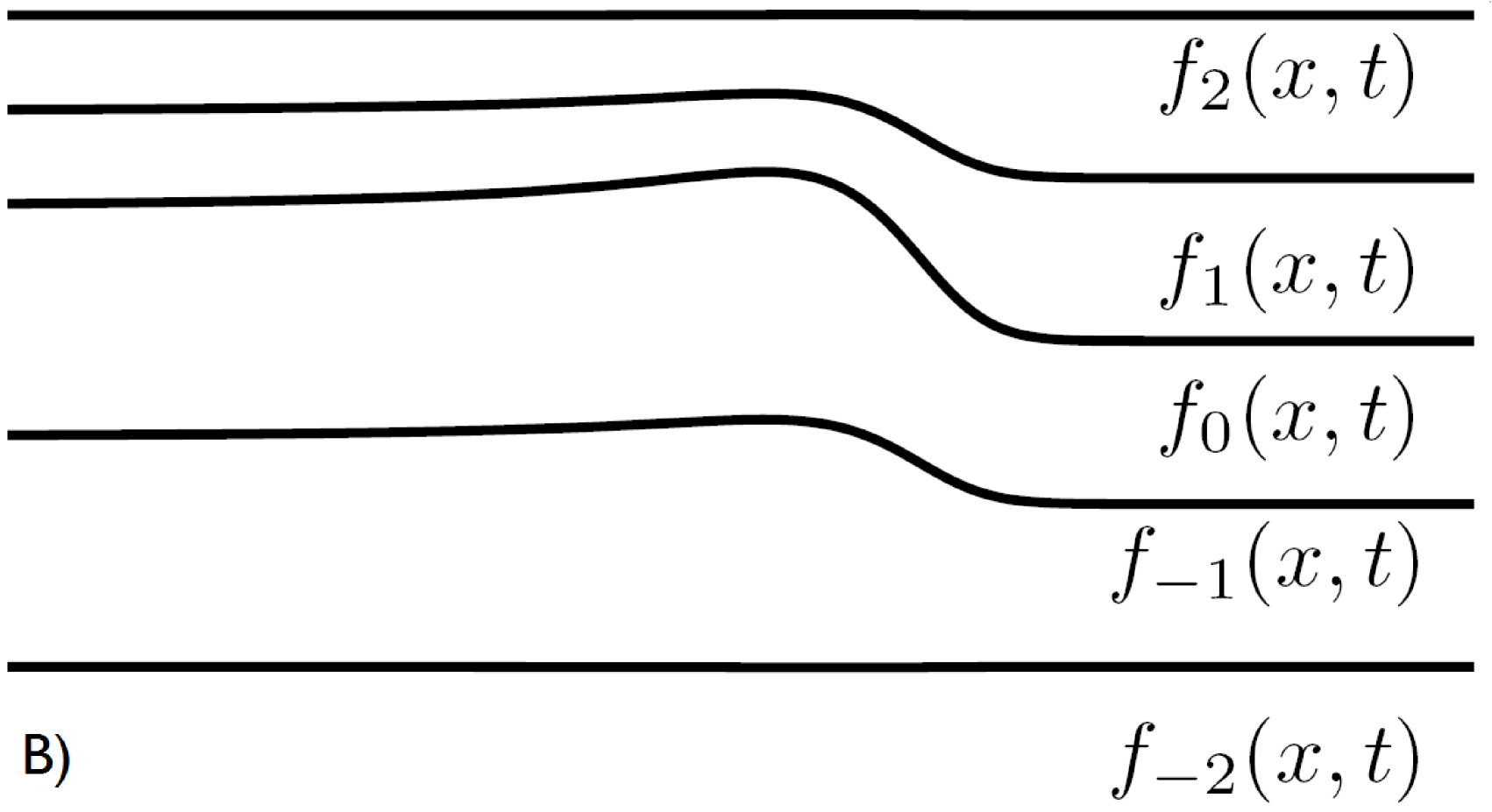
	$\downarrow$    LBM    $\downarrow$
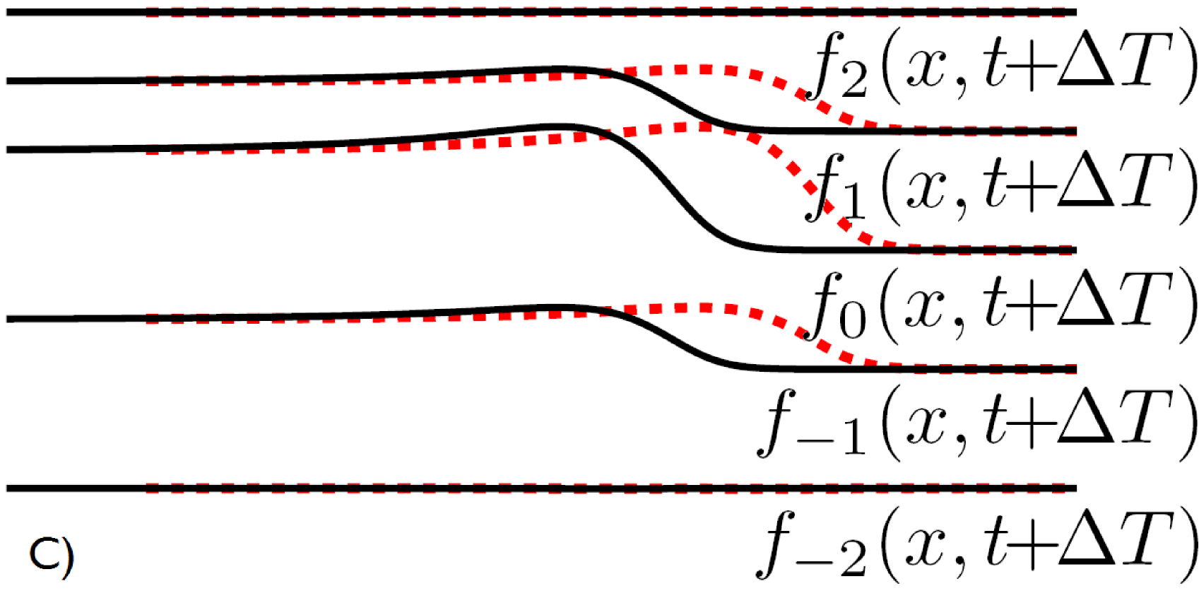
$\uparrow$ LIFT $\uparrow$		$\downarrow$ RESTRICT $\downarrow$
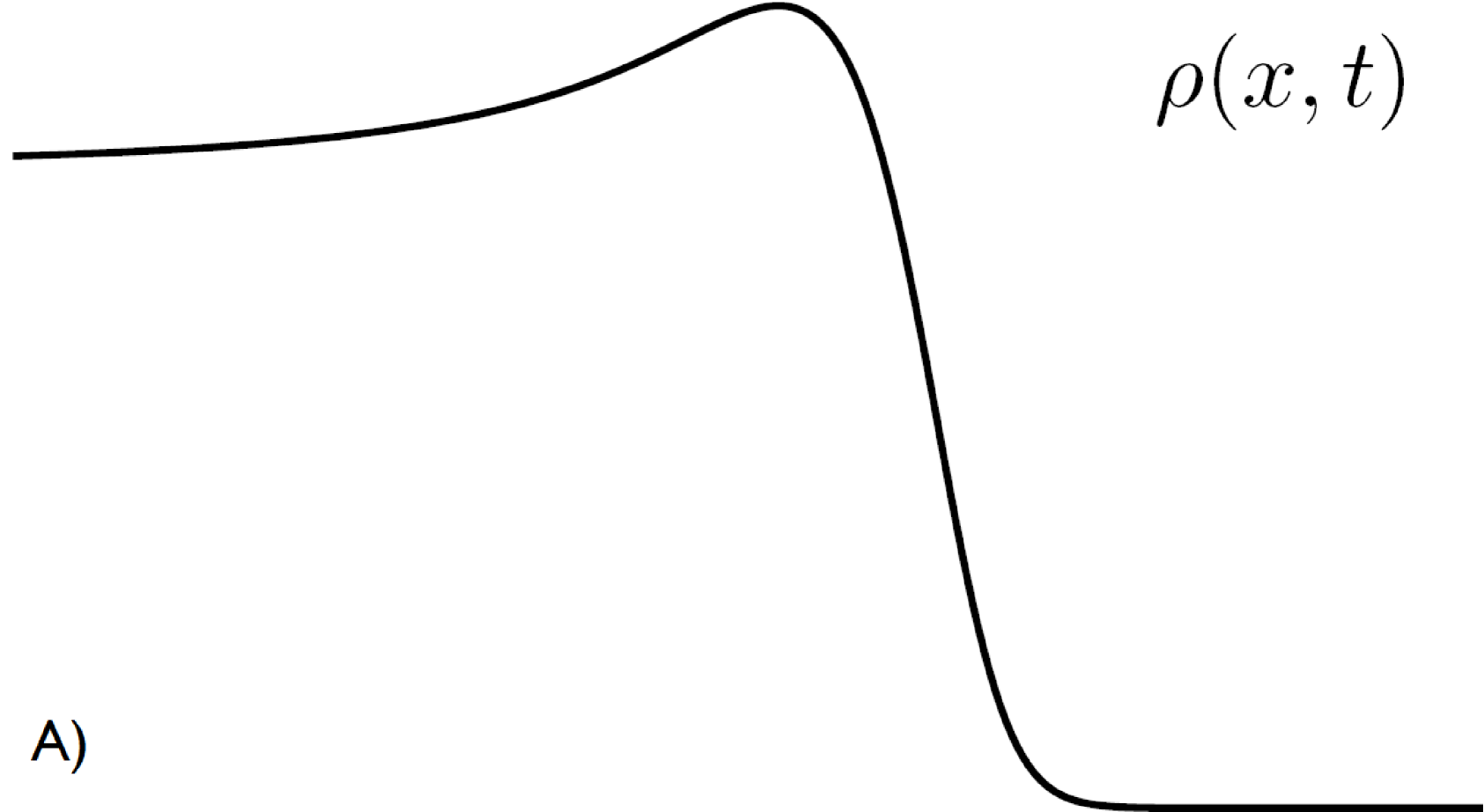
	$\uparrow$   SHIFT-BACK   $\uparrow$

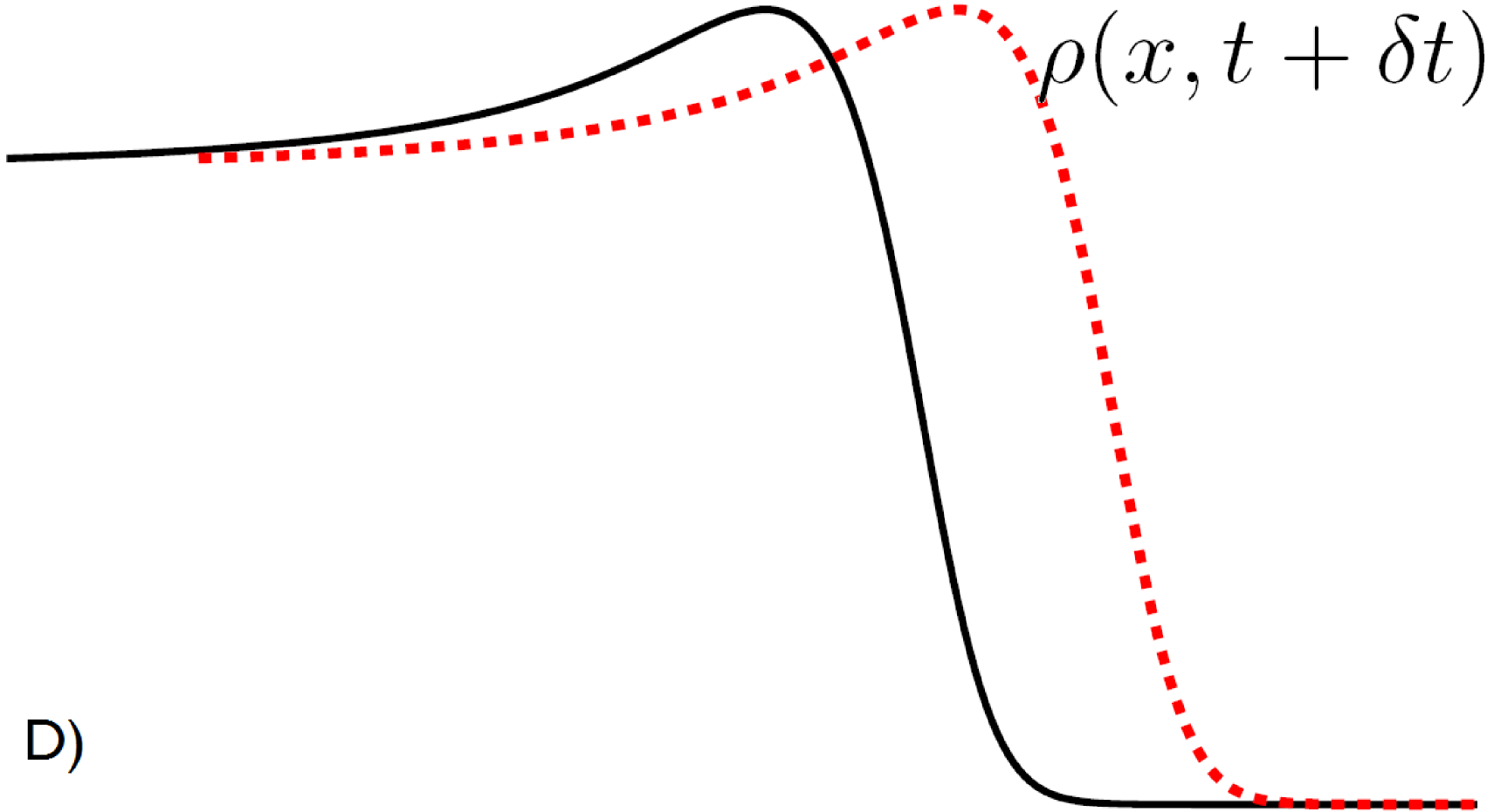
Figure 3: A summary of the different steps involved in finding the traveling wave solutions as fixed points of the coarse-grained time-stepper. We start with an initial guess for the density in the left bottom (panel a). This density is mapped to the corresponding components of the one-particle distribution function using the constrained runs lifting operator. The initial conditions (panel b) are then evolved with the full lattice Boltzmann model over a time $\Delta T$. Each component travels over a distance $c\Delta T$ and arrives at panel c. In the next step, the density at time $t+\Delta T$ is extracted using the restriction operator (panel d). The resulting density is shifted back over a distance $c\Delta T$ to arrive at the original position. The traveling wave solution should be invariant under this sequence of operations and is formulated as a fixed point.

In this section, we describe an alternative way to perform the analysis of the macroscopic behavior of the system. It is based on the work of Kevrekidis et al. manifesto who developed a coarse-grained time stepper (CGTS), which is an effective evolution law for the density. This evolution law $\mathcal{F}$ is not an analytic expression such as a PDE, but the following sequence of computational steps: 1) lifting, 2) simulation and 3) restriction, denoted by the operators $\mu$, LBM and $\mathcal{M}$ respectively (figure 3). Note that the simulation time $\Delta T$ is in general a multiple of $\Delta t$, the lattice Boltzmann time step. Formally, this is written as

$$U(x,t+\Delta T) = \mathcal{F}(U(x,t),\Delta T)$$ (53)

$$= \mathcal{M}(\mbox{LBM}(\mu(U(x,t)),\Delta T)),$$

where we have introduced $U(x,t)=(\rho(x,t),E(x,t))$ as a shorthand notation. The time-stepper $\mathcal{F}$ evolves the macroscopic density $\rho(x,t)\!=\!\sum_{i\in\mathcal{S}}f_{i}(x,t)$ and the electrical field $E(x,t)$ from time $t$ to $t+\Delta T$.

V.1 Lifting

Since the electrical field $E(x,t)$ is the same in both the lattice Boltzmann and the macroscopic model, we can ignore it for the discussion of the lifting and restriction operators. In the lifting step, the particle distribution functions are initialized starting from the initial density

$$\mu:\mathbb{R}^{n}\mapsto\mathbb{R}^{n\times m}:\rho(x_{j},t)\mapsto f_{i}(x_{j},t)$$

with $i\in\mathcal{S}$, $m$ the number of speeds in $\mathcal{S}$, and $j\in\{1,2,\ldots,n\}$ denoting the discrete spatial grid points. Because lifting is a one-to-many mapping problem, it is the most critical step in the coarse-grained time-stepper. We use the constrained runs scheme, an algorithm proposed in gear in the context of singularly perturbed systems. Here, it is wrapped around a single time step $\Delta t$ of the lattice Boltzmann model pvl .

The procedure is given in table 1.

  Algorithm 1 Constrained runs scheme for LBM   initialize $f_{i}^{[0]}=w_{i}^{eq}\rho(x,t)$ $\forall i\in\mathcal{S}$ repeat $f^{[k+1]}=\mbox{LBM}(f^{[k]})$ a single LBM step $\varrho^{[k+1]}=Mf^{[k+1]}$ map into moments $\rho^{[k+1]}=\rho(x,t)$ reset the density $f^{[k+1]}=M^{-1}\varrho^{[k+1]}$ map into distributions until convergence heuristic  

Table 1: Lifting. The constrained runs algorithm computes the distribution functions $f_{i}(x,t)$ corresponding to a given density $\rho(x,t)$. The superscript $k$ indicates the iteration number.

Starting from an initial guess $\rho(x,t)$ for the density, we obtain initial guesses for the distribution functions using the BGK equilibrium weights (8). This choice determines the initial guess for the higher order moments through the transformation matrix $M$, see equation (23). (In principle, the initial guesses for the higher order moments can be chosen arbitrarily; the scheme is designed precisely to converge to the correct value of these moments for the given density.)

We then perform the following iteration. First, we use the lattice Boltzmann model to evolve $f_{i\in\mathcal{S}}^{[k]}$ from $t$ to $t+\Delta t$. The result is transformed back into the moment representation by a matrix multiplication with $M$, which gives us $\varrho^{[k+1]}$. Next, the zeroth moment of the vector $\varrho^{[k+1]}$ is reset to the initial value $\rho(x,t)$. Transforming this modified moment vector $\varrho^{[k+1]}$ back into distribution functions gives us the next $f_{i\in\mathcal{S}}^{[k+1]}$. We repeat this iteration until the higher order moments have converged.

Figure 4: Convergence of the constrained runs algorithm for the five speed ionization model both during lifting and simulation step. Top: Error (2-norm) in the lifted distribution functions (circles) and the flux (squares) as a function of the number constrained runs iterations. After an initial convergence with rate $|1-1/\tau-\Delta tR|$, the error stagnates after approximately 25 iterations. Bottom: Difference (2-norm) between the distribution functions (circles) and the flux (squares) of the lattice Boltzmann simulation that started from the stagnation point of the top figure and the original simulation. Again the error decreases for approximately 25 lattice Boltzmann steps. Note however that after stagnation there is a slow evolution because the macroscopic fields also evolve.

The convergence behavior of the constrained runs algorithm from table 1 is analyzed in pvl for one-dimensional reaction-diffusion lattice Boltzmann models with $\mathcal{S}=\{-1,0,1\}$ (D1Q3 stencil) and a density dependent reaction term. For such systems, the algorithm is unconditionally stable and converges up to the first order terms in the Chapman-Enskog expansion of the distribution functions. The convergence rate is $|1-1/\tau|$, i.e. the same rate at which the lattice Boltzmann simulation relaxes towards the diffusive BGK equilibrium.

Below, we extend the results from pvl to the current five speed model with the velocity dependent reaction term (11). In the absence of an electrical force field, the distributions $f_{\pm 2}$ for the fast particles evolve as (20), i.e.

$$f_{\pm 2}(x_{j}\pm 2\Delta x,t+\Delta t) = (1-\frac{1}{\tau}-\Delta tR)f_{\pm 2}(x_{j},t)$$ (54)

$$+ \frac{1}{\tau}w^{eq}_{\pm 2}\rho(x_{j},t),$$

where the second term is “frozen” because in each iteration of the constrained runs algorithm, the density is reset to its original value. Because the LBM propagation of distributions is a conservative operation succi , this iteration is linearly stable if

$$|1-\frac{1}{\tau}-\Delta tR|<1.$$ (55)

The distributions $f_{\pm 1}$ evolve as

$$f_{\pm 1}(x_{j}\pm\Delta x,t+\Delta t)=(1-\frac{1}{\tau})f_{\pm 1}(x_{j},t)$$ (56)

$$+ \frac{1}{\tau}w^{eq}_{\pm 1}\rho(x_{j},t)+\Delta tR\big{(}f_{+2}(x_{j},t)+f_{-2}(x_{j},t)\big{)},$$

where the number of slow particles is increased proportional to the number of fast particles because of the ionization reaction. Again, the density value in the BGK equilibrium in (56) is “frozen” to the initial value. Because the convergence rate for the $f_{\pm 2}$ components is given by (55), equation (56) converges at a rate $|1-1/\tau-\Delta tR|$ if this value dominates over $|1-1/\tau|$, or at a rate $|1-1/\tau|$ if the latter is dominant over (55).

So far, we have no formal proof for the convergence when an electrical field is present, but we can illustrate the convergence of the algorithm for the full system (20)–(21) numerically for the parameter settings from section VII. The figure is produced as follows. We first extract the velocity moments (22) from a full lattice Boltzmann simulation that has evolved from an initial state for several thousand time steps. Subsequently, we use the obtained density $\rho$ as the initial condition for another lattice Boltzmann simulation and use algorithm 1 for its initialization; the distribution functions of the original simulation are considered to be the “exact” solution. Figure 4 (top) plots the norm of the error between the constrained runs state and the state of the first lattice Boltzmann simulation that it tries to reconstruct. We also observe that after initialization, when evolving the full lattice Boltzmann system both from the “exact” and the re-initialized distributions, the error between the first and second system further decreases (figure 4, bottom). The same observation was made in samaey . Note that we have no analytical expression for the initial state returned by the constrained runs scheme in this setting, but we believe that the results on the accuracy from pvl generalize and that the obtained initial state is a first order approximation of the Chapman-Enskog relations.

V.2 Simulation

In the simulation step, the initial distributions obtained from the lifting step, are evolved for a coarse-grained macroscopic time step $\Delta T$ using the lattice Boltzmann model discussed in the previous sections. This step is denoted as

$$f_{i}(x_{j},t+\Delta T)=\mbox{LBM}(f_{i}(x_{j},t),\Delta T),$$

where the number of time steps depends on the ratio of $\Delta T/\Delta t$. When the ratio is not an integer, a linear interpolation is used between subsequent steps.

V.3 Restriction

In the last step, the restriction step, we extract the macroscopic variables from the result of the simulation. The macroscopic density at time $t+\Delta T$ is then

$$\mathcal{M}:\mathbb{R}^{n\times m}\mapsto\mathbb{R}^{n}:f_{i}(x_{j},t+\Delta T)\mapsto\\ \rho(x_{j},t+\Delta T)=\sum_{i\in\mathcal{S}}f_{i}(x_{j},t+\Delta T).$$ (57)

VI The traveling waves as a fixed point problem

In this section we describe the methodology outlined in samaey to find the traveling wave solutions of the coarse-grained time-stepper $\mathcal{F}(U(x,t))$ defined in section V. If a traveling wave solution with a speed $c$ of $\mathcal{F}(U(x,t))$ is evolved over a time $\Delta T$, the solution has shifted over a distance $c\Delta T$. We define a shift-back operator $\sigma_{\psi}$ that shifts the solution back over a distance $\psi.$

$$\sigma_{\psi}:U(x,t)\mapsto\sigma_{\psi}(U(x,t))=U(x,t)+\psi\partial_{x}U(x,t),$$

where we implement the shift-back by using the characteristic solution of $\partial_{t}U(x,t)+\psi\partial_{x}U(x,t)$ in the forward Euler time discretization.

This shift-back operator is combined with the coarse-grained time-stepper to write a non-linear system for the traveling wave in the co-moving coordinate system with $\xi=x-ct$

$$U(\xi)-\sigma_{c\Delta T}\left(\mathcal{F}(U(\xi),\Delta T)\right)=0.$$ (58)

This equation expresses the sequence of computational steps as illustrated in figure 3. This system, however, is singular because any translate of a solution will also be a solution of (58) samaey .

To get a regular system we add phase (pinning) condition $p(U)$ and a regularization parameter $\alpha$ as an additional unknown, as discussed in samaey . The resulting non-linear system is

$$\mathcal{G}(U,\alpha)=\left\{\begin{array}[]{lcc}U-\sigma_{c\Delta T}\left(\mathcal{F}(U,\Delta T)\right)&=&0\\ p(U)&=&0\end{array}\right.,$$ (59)

where the phase condition $p(U)$ is defined as

$$p(U)=\int_{\xi_{0}}^{\xi_{N-1}}U(\xi)d_{\xi}U_{ref}(\xi)d\xi.$$

This condition minimizes phase shifts with respect to the reference solution $U_{ref}(\xi)$.

VI.1 Preconditioned Newton-GMRES

We solve the non-linear system (59) using a Newton-Raphson method,

$$\left\{\begin{array}[]{lcr}U^{[k+1]}&=&U^{[k]}+dU^{[k]}\\ \alpha^{[k+1]}&=&\alpha^{[k]}+d\alpha^{[k]}\end{array},\right.$$

where the corrections $dU^{[k]}$ and $d\alpha^{[k]}$ are calculated by solving, in each Newton iteration, a linear system of the form

$$\left(\begin{array}[]{cc}I-J(U^{[k]},\alpha^{[k]})&d_{\xi}U^{[k]}\\ d_{U}p(U^{[k]})&0\end{array}\right)\left(\begin{array}[]{c}dU^{[k]}\\ d\alpha^{[k]}\end{array}\right)$$ (64)

$$=-\mathcal{G}(U^{[k]},\alpha^{[k]}).$$ (65)

This system is the linearization of $G(U,\alpha)$ around the point $(U^{[k]},\alpha^{[k]})$ and $J(U^{[k]},\alpha^{[k]})$ denotes the Jacobian of $\sigma_{c\Delta T}(\mathcal{F}(U^{[k]},\alpha^{[k]}))$. Since $\mathcal{F}$ is defined as a sequence of computational steps, it is impossible to construct the Jacobian $J$ explicitly. We therefore use a Krylov method (GMRES) that only requires its application to a vector $v$, which can be estimated as

$$(I-J(U,\Delta T))v\approx\\ v-\frac{\sigma_{c\Delta T}\left(\mathcal{F}(U+\epsilon v,\Delta T)\right)-\sigma_{c\Delta T}\left(\mathcal{F}(U,\Delta T)\right)}{\epsilon}.$$ (66)

Since the convergence rate of GMRES depends sensitively on the spectral properties of the system matrix (65), we propose to precondition the linear system (65) with a rough macroscopic model based on a PDE to speed up the convergence samaey . In section IV, we derived an approximate PDE model using a Chapman-Enskog expansion. We define a time-stepper for this approximate model as $F(U(x,t),\Delta T)$, we can again write a non-linear system

$$G(U,\alpha)=\left\{\begin{array}[]{lcc}U-\sigma_{c\Delta T}(F(U,\Delta T))&=&0\\ p(U)&=&0\end{array}\right.,$$ (67)

in which we have replaced the coarse-grained time-stepper by a time-stepper for the approximate PDE model. The solution of this system will look very similar to the solution of the full model, but will differ in places where the approximations made during the derivation of the PDE model fail.

Figure 5: The traveling wave solution for $c=1.3$ and $R=100$. It is a fixed point of sequential application of the evolution with the coarse-grained time-stepper over a time $\Delta T$ and the shift-back over a distance $c\Delta T$.

The linearization of this problem leads to a matrix problem for the Newton corrections $dU^{[k]}$ and $d\alpha^{[k]}$ as in (65) with very similar spectral properties. The Jacobian however, is now known analytically and can be inverted easily. The idea is to use this matrix as a preconditioner of the linear system that is solved each Newton iteration. The preconditioned system reads

$$\left(M(U^{[k]},\alpha^{[k]})\right)^{-1}A(U^{[k]},\alpha^{[k]})\left(\begin{array}[]{c}dU^{[k]}\\ d\alpha^{[k]}\end{array}\right)$$ (70)

$$=-\left(M(U^{[k]},\alpha^{[k]})\right)^{-1}G(U^{[k]},\alpha^{[k]}),$$ (71)

where $\left(M(U^{[k]},\alpha^{[k]})\right)^{-1}$ is the inverse of the matrix of the linearization of (67) and $A(U^{[k]},\alpha^{[k]})$ denotes the linear system of (65). Because the spectral properties of $A(U^{[k]},\alpha^{[k]})$ and $M(U^{[k]},\alpha^{[k]})$ are so similar that $\left(M(U^{[k]},\alpha^{[k]})\right)^{-1}A(U^{[k]},\alpha^{[k]})$ has spectral properties favorable for the convergence of GMRES. Detailed numerical experiments, showing the spectral properties of the linear systems and the GMRES convergence, are reported in samaey .

VI.2 The minimal speed and the coarse-grained time-stepper

In section IV, we derived the minimal speed $c^{*}$ (52) of the uniformly translating front solution of the PDE model in terms of the asymptotic transport coefficients. Solutions with a speed below this critical value have a density that oscillates in the asymptotic region, which leads to unphysical negative densities.

For the coarse-grained time-stepper, the asymptotic transport coefficients are not available and no analytic expression for the minimal speed can be found. We propose to use the time-stepper and its fixed point solutions to determine the minimal speed. We vary the imposed speed of the shift-back operator $\sigma_{c\Delta T}$ and monitor the solutions of the fixed point problem in the asymptotic region. As the imposed speed $c$ falls below the minimal speed $c^{*}$ the solutions will become oscillatory because the solution in the asymptotic region is a combination of two exponentials (51), whose exponents $\lambda_{\pm}$ coalesce and become complex at the critical speed.

We can extract the two exponents from the solution in the asymptotic region, if we assume that it fits a second order ODE of the form

$$\frac{\partial^{2}\rho}{\partial x^{2}}=a_{1}\rho+a_{2}\frac{\partial\rho}{\partial x}.$$

The coefficients $a_{1}$ and $a_{2}$ are found by taking the fixed point solution in two grid points, where we estimate the spatial derivatives using finite differences. This allows us to formulate a 2-by-2 system for $a_{1}$ and $a_{2}$.

The eigenvalues of the 2-by-2 matrix

$$\left(\begin{array}[]{cc}0&1\\ a_{1}&a_{2}\end{array}\right)$$ (72)

are then $\lambda_{+}$ and $\lambda_{-}$, which coalesce at the critical speed.

For a speed $c$ far above the critical speed $c^{*}$, this method estimates only one of the two exponents with confidence. Indeed, above the critical speed the solution in the asymptotic region is a combination of two decaying exponentials with different exponents. However, one of them is slowly decaying, while the other decays fast. Far away from the critical speed, the method will only detect the slowly decaying exponential and a fit with a first order ODE would be sufficient. Near the critical speed, however, the solution is a combination of both exponentials that decay with comparable rates and both eigenvalues can be reliably extracted from the solution.

VII Numerical Results

As an illustration, we look at a one-dimensional lattice Boltzmann model on a grid with $N=1600$, grid distance $\Delta x=0.4$ and a time step $\Delta t=0.008$. We look at a model with five velocities with ($\mathcal{S}=\{-2,-1,0,-1,2\})$, weights $w_{i}^{eq}=\{0,1/4,2/4,1/4,0\}$ and an electron diffusion coefficient of $D=1.0$. This leads to a relaxation parameter of $\tau=0.8$ or $\omega=1.25$. Note that with this choice of equilibrium weights only slow particles exist in the absence of external fields.

We enforce boundary conditions at the level of the lattice Boltzmann model where we use homogeneous Dirichlet boundaries at the right and no-flux boundaries at the left. The electrical field is kept constant at $E^{+}=-1.0$ at the right and at the left we require that $\partial^{2}E/\partial x^{2}=0$.

We first compute the traveling wave with speed $c=1.30$ for a reaction rate $R=100$, which is shown in figure 5. As an initial guess for the Newton procedure, we take

$$\begin{array}[]{ccc}\rho(x,t)&=&0.025/(1+\exp(0.15(x-L\,2/3)))\\ E(x,t)&=&-1/(1+\exp(0.05(x-L\,5/9)))\end{array}$$ (73)

To assess the overall performance of the method, we compute the total number of required lattice Boltzmann time steps. We observe that about 5 Newton steps are needed. Each Newton step, in turn, requires the solution of a linear system with the help of a preconditioned Krylov subspace. On average about 40 GMRES iterations are required to solve the linear system with a tolerance of $1\cdot 10^{-12}$. Each GMRES iteration requires an evaluation of the CGTS, which costs about 50 lattice Boltzmann iterations — 25 for the lifting and 25 for the simulation. This leads to a total of 10 000 evolutions with the lattice Boltzmann system to find a single fixed point. Detailed figures about convergence are given in samaey .

Next, we vary the cross section $R$, which is related to the number of times an ionization reaction appears, and study the effect on the critical velocity of the traveling wave solution. We increase $R$ from 60 to 100, which corresponds at the level of the PDE to an increase of the growth transport coefficient from $\alpha(E^{+})=0.02015$ to $\alpha(E^{+})=0.03707$, with $E^{+}=-1.0$. For this range of reaction rates with the chosen value of $\Delta t$, the constrained runs algorithm always converges because all the eigenvalues of the Jacobian are smaller than $|1-1/\tau-\Delta tR|<1$, as discussed in section V.1.

We now turn to the numerical computation of the critical velocity with the method proposed in section VI.2. In table 2, we show the critical speed determined for a series of ionization strengths between $R=60$ and $R=100$. As outlined in section VI.2, the critical velocity for each value of $R$ is found by performing a numerical continuation with the wave speed $c$ as a free parameter and monitoring the eigenvalues of the 2-by-2 matrix (72). For comparison, we also show the minimal speed as obtained using the approximate analytical expressions for the transport coefficients, which we found through the Chapman-Enskog expansion. We observe a small difference between the two results. The critical speed that results from the Chapman-Enskog expansion is higher than the critical speed that is computed using the CGTS. Note that both methods make approximations and it is not clear which method is more exact.

A short discussion about the accuracy of the shift-back operator is necessary. Since we have implemented the shift-back operator using a forward Euler approximation of the characteristic solutions of the equation $u_{t}+cu_{x}=0$, the error in the critical speed grows linearly with the time step $\Delta T$. Therefore, we should take $\Delta T$ as small as possible, i.e.  the minimal possible number of lattice Boltzmann steps in the simulation step. (Note that accuracy and efficiency go together here.) However, we cannot take less than 25 LBM steps because these steps are necessary to reduce the error in the lifting (see figure 4).

$R$	$c^{*}$ with	$c^{*}$ with
	Chapman-Enskog	CGTS
60	1.3351	1.3177
70	1.3496	1.3318
80	1.3609	1.3433
90	1.3696	1.3517
100	1.3755	1.3566

Table 2: The critical speed for different values of the ionization rate $R$.

VIII Discussion and Conclusions

In one dimension, an initial seed of electrons in a strong electrical field will evolve into a streamer front that travels with a constant speed $c$. Before the front, the density is zero and the electrical field is constant; behind the front the electrical field is shielded and there is a surplus of electrons. In this article we extended the minimal streamer model of Ebert et al. ebert to add some details about the microscopic physics. To this end, we replaced the reaction-diffusion PDE with a lattice Boltzmann model that has a velocity dependent reaction term. The reaction rates are a chosen to model the ionization reaction, where fast particles have a given probability to undergo an ionization reaction and create two slow particles. The electrical field changes simultaneously as a result of the charge creation.

This macroscopic behavior of the model was analyzed with two methods. The first is the more traditional analysis based on a Chapman-Enskog expansion that derives an approximate PDE model and the corresponding transport coefficients. The resulting PDE model is very similar to the minimal streamer model of Ebert, Van Saarloos and Caroli, where the ionization rate depends on the local electrical field. Based on the transport coefficients, we found the dependence of the critical speed (below which the traveling waves are unphysical) and its dependence on the strength of the ionization cross section.

Our second method is a computational method based on the coarse-grained time-stepper, which defines the effective evolution law as a sequence of computational steps. The traveling wave solutions were formulated as fixed points of this coarse-grained time-stepper combined with a shift-back operator. By varying the applied shift-back, we again found the critical speed, and we demonstrated how to calculate its dependence on the cross section strength numerically.

We showed that the coarse-grained time-stepper provides a viable alternative to the traditional Chapman-Enskog analysis. However, in this paper, we did not make any statements about which of the two methods provides the most accurate information. Both methods make approximations to obtain the critical velocity of the proposed lattice Boltzmann model. In contrast to the theoretical approximations in the Chapman-Enskog analysis, these approximations are due to numerical accuracy for the coarse-grained time-stepper.

Further progress in the accuracy can be made in several ways. First, the lifting can be done more accurately if a higher order constrained runs algorithm is used. Such a method would take multiple steps with the lattice Boltzmann model and uses these multiple points to provide us with an approximate initial state gear . We expect that these higher order lifting procedures will reproduce more than two terms in the Chapman-Enskog series and therefore provide a better initial state for the simulation step. This will allow limiting the number of simulation steps, which will immediately improve the accuracy of the computed solutions and the critical speed.

Although the model problem in this paper is non-trivial, and the Chapman-Enskog expansion is tedious, we emphasize that our method is mainly developed with applications in sight where the traditional Chapman-Enskog analysis is completely intractable. The model problem in this paper both allows us to analyze the proposed methods and provide directions for further development. In a forthcoming article, we will do a complete analysis of the traveling wave solutions in the proposed model and illustrate more extensively how the macroscopic behavior depends on the parameters of the microscopic model. In our calculations, we have also observed the positively charged fronts that move in the opposite direction of the electrical field. These solutions have been discussed by Ebert et al in ebert and our methods are also able to locate these states.

We expect that most of the results presented in this paper will remain valid when the number of velocities in the discretization of the Boltzmann model is increased. With additional velocities, it is possible to model the cross sections of colliding particles with more detail and study other reactions than the ionization reaction. It would also be interesting to study models with multiple species where the collision rates between the particles are velocity dependent. This would allow us to include photo-ionization effects into the minimal streamer model, an important effect that is neglected in the current model kuli .

- (1) U. Ebert, W. Van Saarloos, and C. Caroli, Phys. Rev. E, 55 p1530 (1997).
- (2) W. Van Saarloos, Phys. Rep. 386 p29-222 (2003).
- (3) G. Samaey, W. Vanroose, D. Roose and I.G. Kevrekidis, Coarse-grained computation of traveling waves of lattice Boltzmann models with Newton-Krylov methods, submitted to Journal of Computational Physics, (2006). Arxiv preprint physics/0604147.
- (4) P. Van Leemput, W. Vanroose and D. Roose, Initialization of a lattice Boltzmann model with constrained runs, submitted. Technical Report TW 444, Dept. of Computer Science, K.U.Leuven (2005).
- (5) I. G. Kevrekidis et al, Comm. Math. Sci. 1 p715 (2003).
- (6) W. Hu, D. Fang, Y. Wang and F. Yang, Phys. Rev. A, bf 49 p 989 (2006)
- (7) T. N. Rescigno, M. Baertchy, W. A. Isaacs and C. W. McCurdy, Science 5449 p2474 (1999).
- (8) M. S. Pindzola and D. R. Schultz. Phys. Rev. A 53 p1525 (1996).
- (9) L. Malegat, P. Selles, and A. K. Kazansky, Phys. Rev. Lett 85 p4450 (2000).
- (10) I. Bray and A. T. Stelbovics, Phys. Rev. A 46 p6995 (1992).
- (11) W. Vanroose, F. Martin, T. N. Rescigno and C. W. McCurdy, Science, 310 p5755 (2005).
- (12) T. Weber et. al., Nature 7007 p437-439 (2004).
- (13) G. H. Wannier, Phys. Rev. 90 817 (1953).
- (14) N. Cao, S. Chen, Shi Jin and D. Martinez, Phys. Rev E, 55, R21 (1997).
- (15) A. Arnold and C. Ringhofer, SIAM Journal of Numerical Analysis, 33 p1622 (1996).
- (16) S. Succi, The lattice Boltzmann equation for fluid dynamics and beyond, Oxford University Press (2001).
- (17) C. W. Gear, T. J. Kaper, I. G. Kevrekidis, and A. Zagaris. Projecting to a slow manifold: Singularly perturbed systems and legacy codes. SIAM Journal on Applied Dynamical Systems, 4 p711, (2005).
- (18) G. E. Uhlenbeck and G. W. Ford, Lectures in Statistical Mechanics, American Mathematical Society, Providence, Rhode Island, (1963).
- (19) Y.H. Qian, D. d’Humières, and P. Lallemand, Lattice BGK models for the Navier-Stokes equation. Europhysics Letters, 17 p479 (1992).
- (20) L. Qiao, R Erban, C.T. Kelley, I. G. Kevrekidis, Spatially distributed Stochastic Systems: Equation-free and equation-assisted bifurcation analysis submitted to Phys. Rev. E, arxiv preprint q-bio/0606006.
- (21) P. L. Bhatnagar, E. P. Gross and M. Krook, Phys. Rev. 94, p511 (1954).
- (22) A. A. Kulikovsky, Phys. Rev. Lett. 89 p229401 (2002)