Atom interferometry using wavepackets with constant spatial displacements

Abstract

We demonstrate a standing-wave light pulse sequence that places atoms into a superposition of wavepackets with precisely controlled displacements that remain constant for times as long as 1 s. The separated wavepackets are subsequently recombined resulting in atom interference patterns that probe energy differences of $\approx 10^{-34}$ Joule, and can provide acceleration measurements that are insensitive to platform vibrations.

I Introduction

Atom interferometry employs the interference of atomic de Broglie waves for precision measurements AIBerman . In practice two effects limit the ultimate sensitivity of devices where the interfering atomic wavepackets are allowed to propagate in free space: the effect of external gravitational fields upon the atomic trajectories, and transverse expansion of the atom cloud. By accounting for gravity, atomic fountains can increase the interrogation time during which the interferometry phase shifts accumulate Chugravity ; alternatively one can use magnetic dipole forces to balance the force of gravity Clauser88 . Magnetic waveguides CornellGuide99 ; PrentissGuide2000 can trap atoms for times longer than a second, suggesting the possibility of measuring energy differences between interfering wavepackets with an uncertainty $<\hbar$/(1 s)$\sim 10^{-34}$ Joule; however, this remarkable precision cannot be obtained if the decoherence time of the atoms is much shorter than the trap lifetime. Early atom interferometry experiments using atoms confined in magnetic waveguides showed that the external state coherence of the atoms decayed quite quickly, limiting interferometric measurements to times $<$10 ms Wang et al. (2005); Wu et al. (2005a). More recent experiments using Bose condensates Jo et al. (2007) have shown that the external state coherence can be preserved for approximately 200 ms, where the decoherence is dominated by atom-atom interactions. Interferometry experiments using either condensed atoms in a weak trap, or using non-condensate atoms in a waveguide with precise angular alignments have been shown to have phase-stable interrogation time of $\approx 50$ ms, where the dephasing is induced by inhomogeneities in the confining potential. Garcia et al. (2006); Burke08 ; Burke09 ; Wu et al. (2007).

This work demonstrates a new atom interferometer configuration that measures the differential phase shift of spatially-displaced wavepacket pairs. We demonstrate phase-stable interferometry operations with up to one second interrogation time by applying the technique to atoms in a straight magnetic guide. We show that the matter-wave dephasing rate scales linearly with the wavepacket displacement, suggesting that dephasing in our interferometer is primarily caused by a weak longitudinal confinement of the atoms. We also demonstrate that the phase readout of the interferometer is less sensitive to vibration than conventional interferometery schemes, which should enable precision measurements even in noisy environments such as moving platforms.

Figure 1: (Color online) Recoil diagram of the 4-pulse scheme. The light shift potential of the standing wave is represented by the array of circles. Straight lines show the centers of the diffracted wavepackets. A representative pair of interfering paths is marked with thick lines. The matter-wave interference at around $t=T$ is probed with $E^{a}$. The backscattered light, e.g., the “grating echo” $E^{b}(\tau)$, is mixed with a weak local field from $E^{b}$ mode for phase retrieval.

II The 4-pulse grating echo scheme

Typical Talbot-Lau matter-wave interferometery ClauserInftheory92 ; Cahn et al. (1997); Strekalov et al. (2002); Brezger et al. (2002) employs a 3-grating diffraction scheme. In the most common time-domain setup, an atomic wavepacket is diffracted by a periodic potential, applied briefly at time $t=0$, into a collection of wavepackets that depart from each other at multiples of the velocity ${\bf v}_{\bf Q}=\hbar{\bf Q}/m$, where ${\bf Q}$ is the potential’s wavevector and $m$ is the atomic mass. The potential is pulsed on again at $t=T/2$, and the different velocity classes created by the first pulse, which have now moved away from each other, are each again diffracted into multiple orders. After the second pulse there will be pairs of wavepackets whose relative velocity has been reversed from before; these will move toward each other, then overlap and interfere near time $t=T$. Those with relative velocity $n{\bf v}_{\bf Q}$ will generate density fringes with wavevector $\pm n{\bf Q}$.

As in earlier experiments Cahn et al. (1997); Mossberg et al. (1979) we use an off-resonant optical standing wave (SW) to create the pulsed periodic potentials, and observe the resulting atomic density fringes by measuring the Bragg scattering of an optical probe. In our experiment we observe the lowest order fringes, $n=\pm 1$, where the Bragg condition corresponds approximately to backscattering of one of the beams that forms the standing wave.

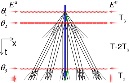
The interferometric technique presented here employs a 4-pulse scheme (Fig. 1), where the additional pulse is used to halt the relative motion of the interfering wavepacket pairs. After the first pulse is applied the situation is identical to that in the 3-pulse case, with the original wavepacket split into different diffraction orders corresponding to velocities $\pm n{\bf v}_{\bf Q}$. Here we quickly apply a second pulse after a short time $t=T_{s}$. The pairs of wavepackets that we are interested in, those that will eventually interfere, are those that now have zero momentum difference; these pairs have the same velocity but are displaced in space, having moved apart by a distance (${\bf d}={\bf v_{Q}}T_{s}$) during the interval between pulses. After waiting for a time $T-2T_{S}$ the coherence between the wavepackets is measured by allowing them to interfere; a third pulse diffracts the wavepackets at $t=T-T_{s}$ and the resulting interference fringe is probed around $t=T$. This 4-pulse sequence can be imagined as a 3-pulse sequence of length $2T_{s}$ that is ”paused” between times $T=T_{S}$ and $T-T_{S}$; though during this time the relative phase of each separated wavepacket pairs will continue to be sensitive to external fields.

The existing theory of Talbot-Lau interferometry can be straightforwardly extended to this scheme. We consider the SW field formed by the traveling light fields $E^{a}$ and $E^{b}$ with associated k-vectors ${\bf k}^{a}$ and ${\bf k}^{b}$, with ${\bf Q}={\bf k}^{a}-{\bf k}^{b}=Q{\bf e_{x}}$. Experimentally, we measure the backscattering of light from ${\bf k}^{a}$ into ${\bf k}^{b}$; this is characterized by an electric field component $E^{b}(\tau)$ that can be expressed in terms of the atomic density operator:

$$E^{b}(\tau)=-igE_{p}{\rm Tr}[\hat{\rho}(T)e^{iQ(\hat{x}+\frac{\hat{p}\tau}{m})}].$$ (1)

Here $E_{p}$ gives the amplitude of probe light from the $E^{a}$ mode, $g$ is a constant that depends on the atomic polarizability and the number of atoms participating in the interaction, $\hat{x}$ and $\hat{p}$ are the position and momentum operators for atomic motion along $\bf e_{x}$, and $\hat{\rho}(T)$ is the single atom density matrix at time $T$. Consider an atomic sample with a rms velocity $u$ and a thermal de Broglie wavelength $l_{c}=\hbar/(mu)$, in Eq. (1) we use $\tau\sim l_{c}/v_{Q}$ to specify a coherence-length-dependent time window $(T-l_{c}/v_{Q},T+l_{c}/v_{Q})$ during which the atomic wavepackets overlap so that the interference fringe contrast is non-zero. Experimentally, the amplitude of $E^{b}(\tau)$ is averaged during this time window to extract the magnitude of the interference fringe; this will be referred to as the amplitude of the “grating echo”, $E_{g}(T_{s},T):=<E^{b}(\tau)>_{\tau}$ Wu (2007).

For a SW pulse in the Raman-Nath regime, where the atomic motion can be neglected for its duration, the $n^{th}$ order matter-wave diffraction is weighted by the amplitude $i^{n}J_{n}(\theta)$, with $J_{n}$ the $n^{th}$ order Bessel function and $\theta$ the time-integrated light shift or pulse area. We define $\{T_{1},T_{2},T_{3},T_{4}\}=\{0,T_{s},T-T_{s},T\}$, and specify the position of standing wave nodes at $T_{i}$ with the SW phase $\varphi_{i}$. The interaction of the first three SW pulses in the 4-pulse interferometer can be effectively described by

$$\hat{V}_{\rm SW}(t)=\hbar\sum\nolimits_{i=1}^{3}\theta_{i}\delta(t-T_{i})\cos(Q\hat{x}+\varphi_{i}).$$ (2)

Since the standing wave phases $\varphi_{i}$ involve simple algebra, we will ignore them during the following discussion, and reintroduce them when they become relevant.

In order to account for imperfections in the guide we consider the 1D motion of atoms along $\bf e_{x}$ during the interferometry sequence to be governed by $\hat{H}=\hat{H}_{0}+\hat{V}_{\rm SW}(t)$ and further $\hat{H}_{0}=\hat{p}^{2}/2m+V(\hat{x})$ where $V(\hat{x})$ is a general 1D potential. We introduce the time-dependent position and momentum operators $\hat{x}(t)=e^{i\hat{H}_{0}t}\hat{x}e^{-i\hat{H}_{0}t}$ and $\hat{p}(t)=e^{i\hat{H}_{0}t}\hat{p}e^{-i\hat{H}_{0}t}$. For $T_{s}$ to be sufficiently short, the atomic motion can be treated as free during $0<t<T-T_{s}$ and $T-T_{s}<t<T$. For a thermal atomic sample with $Ql_{c}<<1$, we find at the leading order of $Ql_{c}$, the interferometer output is related to the initial atomic density matrix $\hat{\rho}(0)$ by

$$\begin{array}[]{l}E_{g}(T_{s},T)=-igE_{p}J_{-1}(2\theta_{3}\sin\omega_{Q}T_{s})\times\\ \sum\limits_{m_{1},m_{2}}c_{m}{\rm Tr}[\hat{\rho}(\delta x_{m},\delta p_{m},0)e^{\frac{i}{\hbar}d\hat{p}(T)}e^{-\frac{i}{\hbar}d\hat{p}(0)}].\\ \end{array}$$ (3)

Here $c_{m}=J_{m_{1}}(\theta_{1})J_{m_{1}+1}(\theta_{1})J_{m_{2}}(\theta_{2})J_{m_{2}-1}(\theta_{2})e^{i\phi_{m}}$, $\phi_{m}=(2m_{1}+1)Ql_{c}+(2m_{2}-1)\omega_{Q}T_{s}$, $\delta x_{m}=m_{1}v_{Q}T_{s}$, $\delta p_{m}=(m_{1}+m_{2})Q$. In Eq. (3) $\omega_{Q}$ is the two-photon recoil frequency of atoms and we have $d=v_{Q}T_{s}$.

The second line of Eq. (3) composes a weighted sum of matter-wave correlation functions. The initial conditions of matter-wave states are specified by a density matrix $\hat{\rho}(\delta x,\delta p,0)=e^{i(\delta x\hat{p}+\delta p\hat{x})}\hat{\rho}e^{-i(\delta x\hat{p}+\delta p\hat{x})}$ that describes an atomic ensemble that is identical to $\hat{\rho}(0)$, but with mean position and momentum shifted by $\delta x$ and $\delta p$ respectively. The correlation function gives the average overlap of wavepacket pairs propagating under an external potential displaced by $d\bf e_{x}$, with one example sketched with the thick lines in Fig. 1. The correlation functions are in direct analogy to the neutron scattering correlation function discussed in ref. Petitjean et al. (2007) where momentum displacements were considered. Notice that if the uniform atomic sample has a spatial extension $L>>\delta x$ and with thermal velocity $u>>\delta p/m$, the original and shifted density matrix are approximately the same, and the correlation functions are approximately independent of $\delta x_{m}$ or $\delta p_{m}$. We can thus use a sum rule of Bessel functions to simplify the second line of Eq. (3) giving:

$$\begin{array}[]{l}E_{g}(T_{s},T)\approx-i\tilde{g}J_{-1}^{2}(2\theta_{2}\sin\omega_{Q}T_{s})\times\\ {\rm Tr}[\hat{\rho}(0)e^{\frac{i}{\hbar}d\hat{p}(T)}e^{-\frac{i}{\hbar}d\hat{p}(0)}],\end{array}$$ (4)

where we have chosen $\theta_{2}=\theta_{3}$ and define $\tilde{g}=gE_{p}\theta_{1}Ql_{c}$.

Three features of Eq. (3) and Eq. (4) are worth noting:

First, though we have only considered the 1D motion of atoms in the external potential $V(x)$, the formula is readily applicable to a 3D time-dependent potential $V({\bf r},t)$ as long as the external potential contributes negligibly to the differential phase shift of wavepacket pairs during $0<t<T_{s}$ and $T-T_{s}<t<T$.

Second, the reduction from Eq. (3) to Eq. (4) requires that the correlation functions be insensitive to momentum transferred by the SW pulses. This is very well satisfied if the displacements are much smaller than the position and momentum spreadings of the atomic gas itself since $\hat{\rho}(\delta x,\delta p,0)\approx\hat{\rho}(0)$. In addition, the approximation is particularly well satisfied if the potential is periodic at small wavelengths Moore et al. (1995); stability08 .

Finally, notice that both Eq. (3) and Eq. (4) can be evaluated semi-classically by replacing ${\rm Tr}[\hat{\rho}(0)e^{\frac{i}{\hbar}d\hat{p}(T)}e^{-\frac{i}{\hbar}d\hat{p}(0)}]$ with $<e^{\frac{imd}{\hbar}[v(T)-v(0)]}>_{c}$, where $v(t)$ gives the classical velocity of atoms along $\bf e_{x}$ and $<...>_{c}$ gives the classical ensemble average over the atomic initial conditions.

Now consider a weak quadratic potential $V(x)=max+\frac{1}{2}m\omega_{l}^{2}x^{2}$ with an acceleration force $ma$ and with $\omega_{l}T<<1$ to model the potential variation along the nearly free (axial) direction of propagation in the magnetic guide, also assuming an atomic sample with a Gaussian spatial distribution along $\bf e_{x}$ given by $\rho(x)=e^{-x^{2}/(2L^{2})}$. The expected amplitude of the grating echo signal is then found to oscillate with $T_{s}$ and to decay as a Gaussian with the total interrogation time $T$:

$$\begin{array}[]{l}E_{g}(T_{s},T)\approx-i\tilde{g}J_{-1}^{2}(2\theta_{2}\sin\omega_{Q}T_{s})\times\\ e^{-\frac{1}{2}(\frac{md}{\hbar}\omega_{l}^{2}TL)^{2}}e^{i(\frac{md}{\hbar}aT+\varphi_{1,2}-\varphi_{3,4})}.\end{array}$$ (5)

(Here we have reintroduced the standing wave phase in Eq. (2), where $\varphi_{i,j}=\varphi_{i}-\varphi_{j}$)

Figure 2: (Color online) Examples of interferometry signal amplitude $C(T_{s},T)$ oscillation vs $T_{s}$ at fixed $T$. Scatter plots are from experiments. Solid lines are calculated according to an extension of Eq. (5) with complex pulse area $\tilde{\theta}=\theta(1+0.025i)$. (a): $\theta=0.85$ and $T=50$ ms. (b): $\theta=2.8$ and $T=30$ ms. The data were taken during different period of experiments with different signal/noise.

III Experimental setup

The experimental apparatus is described in detail in Ref.  Wu (2007). A straight 2D quadruple magnetic field with a transverse gradient of 70 G/cm is generated by four 200 mm$\times$100 mm$\times$1.56 mm permalloy foils poled in alternating directions. Approximately $10^{7}$ laser-cooled ⁸⁷Rb atoms in the ground state F=1 hyperfine level are loaded into this magnetic guide, resulting in a cylindrically-shaped atom sample 1 cm long and 170 $\rm\mu$m wide. The average transverse oscillation frequency of the atoms in the guide is on the order of 80 Hz, estimated by displacement induced oscillations of the atomic sample using absorption images. A very weak harmonic potential along the guiding direction is estimated to be $\omega_{l}\sim 2\pi\times 0.08$ Hz Wu (2007).

The SW fields formed by two counter-propagating laser beams with diameters of 1.6 mm are aligned to form a standing wave with k-vector along the magnetic guide direction $\bf e_{x}$. Precise angular adjustment is achieved by tuning the orientation of the magnetic guide using two rotation stages to within $2\times 10^{-4}$ radians. The optical fields are detuned 120 MHz above the $F=1$ - $F^{\prime}=2$ D2 transition. We choose the SW pulse with typical pulse area of $\theta\sim 0.8-3.0$, and with duration of 300 ns to be deep in the thin-lens regime of the 25 $\mu$K atomic sample. With this pulse duration, the fraction of atoms contributing to the final interference fringe is typically limited by SW diffraction efficiency to about ten percent. We probe the $\lambda/2$ atomic density grating at around time $t=T$ by turning on only one of the traveling wave beams; the other beam is attenuated and shifted by 6 MHz to serve as an optical local oscillator, where the combined intensity is measured using a fiber-coupled avalanche photodetector. The beat signal is measured and numerically demodulated using the 6 MHz rf reference to recover the grating echo signal $E_{g}(T_{s},T)=C(T_{s},T)e^{i\varphi(T_{s},T)}$. The interferometer signal amplitude $C(T_{s},T)$ and phase $\varphi(T_{s},T)$ are measured for different interferometer parameters.

IV Results and discussions

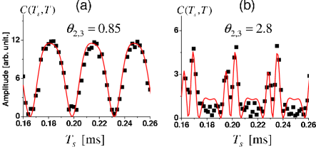
According to Eq. (5), the pre-factor $J_{1}^{2}(2\theta\sin\omega_{Q}T_{s})$ in the backscattering amplitude is an oscillatory function of $T_{s}$, with the periodicity determined by $2\omega_{Q}=2\pi/33.15$ $\rm\mu$s^-1. The amplitude oscillation is reproduced experimentally; two examples are plotted in Fig. 2, where $T_{s}$ is varied from 0.16 ms to 0.26 ms. In Fig. 2(a) a relatively small SW pulse area $\theta\approx 0.85$ was chosen so that the Bessel function is approximately linear. Correspondingly, we see the oscillation is approximately sinusoidal. In Fig. 2 (b) a strong SW pulse with area $\theta\approx 2.8$ was chosen and the Bessel function becomes highly nonlinear. Nevertheless, the experimental data still fits the theoretical expectation from Eq. (5) fairly well. The values for the of pulse area in the calculation were found in agreement with the SW pulse intensity-duration products. Notice the solid lines in Fig. 2 were calculated according to an extension of Eq. (5) with a complex SW pulse area including an imaginary part to account for the optical pumping effect at the 120 MHz SW detuning Wu (2007).

Figure 3: (Color online) (a): Backscattering amplitude decay. The scatter plots give $C(T)$ at four different displacement $d$. The solid lines are due to Gaussian fit. (b): Interferometry phase shift $\varphi(T)$ vs $T$ at different displacement $d$. Four of the data traces from the same experiments as those in (a) are plotted with thick lines.

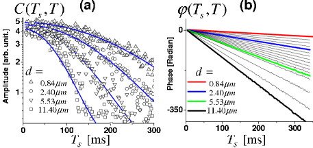
With fixed $T_{s}$ at the peak values of the amplitude oscillations, we now consider the dependence of the interferometer signals on the total interrogation time $T$. Fig. 3 gives examples of the interferometer amplitude decay $C(T)$ and phase shift $\varphi(T)$ at various $d=v_{Q}T_{s}$. From Fig. 3(a) we see the amplitude decay is slower for smaller $d$, while all the $C(T)$ fit fairly well to Gaussian decay, in agreement with Eq. (5) derived from a weak harmonic confinement model. In Fig. 3(b) we see the phase readout is a linear function of interrogation time $T$, also in agreement with Eq. (5). By applying Eq. (5) to the observed phase shifts, we consistently retrieve an acceleration $a=83.4$ mm/s² for different $d$. The acceleration is due to a small component of gravity along the standing-wave/magnetic guide direction $\bf e_{x}$ Wu (2007), as confirmed by varying the tilt angle of the apparatus.

Figure 4: (Color online) (a): Backscattering amplitude decay rate $\gamma(d)$ [extracted from a Gaussian fit of $C(T)$ data such as those from Fig. 3 (a)] vs wavepacket displacement $d$. (b): Interferometry phase shift rate $f(d)=\frac{d\varphi(T)}{dT}$ [extracted from a linear fit of $\varphi(T)$ data from Fig. 3 (b)] vs $d$. The insets give the residuals of the linear fits.

Figure 5: (Color online) Interferometry readouts $C(T)$ and $\varphi(T)$ at $d=0.413$ $\mu$m. (a): $C(T)$ vs $T$; (b): $\varphi(T)$ vs $T$, with inset giving the residual after a linear fit.

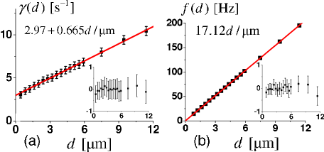
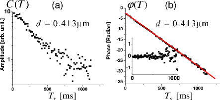
We extract the amplitude decay rate $\gamma(d)$ by fitting the $C(T)$ decay data with $C(T)\propto e^{-(\gamma(d)T)^{2}}$. The dephasing rate $\gamma(d)$ is plotted vs the displacement $d$ in Fig. 4(a). The $d$-dependence of $\gamma(d)$ shows good agreement with a linear fit. According to Eq. (5), for weak confinement along $\bf e_{x}$ with $\omega_{l}\sim 2\pi\times 0.08$ Hz and for $L\sim 2.5$ mm of our 1 cm atomic sample, we expect $\gamma(d)\sim m\omega_{l}^{2}dL/\hbar/\sqrt{2}\sim 0.6d/$ $\mu$m s^-1. This agrees with the experimentally measured $\gamma(d)=(2.97+0.665d/\mu$m) s^-1 according to Fig. 4(a). The offset of $\gamma(d\rightarrow 0)=2.97$s^-1 is partly due to the escape of atoms from the interaction zone via collisions with the walls of the 4 cm vacuum glass cell, which, if fit to a Gaussian, would give $\tilde{\gamma}(d\rightarrow 0)\sim 1.6$ s^-1. The remaining discrepancy is likely due to the inaccuracy of the Gaussian fit which is based on the assumption of a weak harmonic perturbation $V(x)$ in Eq. (5). For small $d$ and thus a small dephasing rate, local anharmonicity in $V(x)$ might become important. Indeed, for long interaction time $T$ the decay exhibits an exponential feature, which is clearly seen in Fig. 5(a) where the amplitude decay $C(T)$ with $d=0.418$ $\rm\mu$m and $T_{s}=35.4$ $\rm\mu$s is plotted. For such a small wavepacket displacement $d$, the phase of the backscattering signal remains stable for $T>1$ s, as shown in Fig. 5(b).

Figure 6: (Color online) Interferometry phase readouts $\varphi(T)$ for a 3-pulse (open triangles, right and top axes.) and a 4-pulse (solid squares, left and bottom axes. $T_{s}=0.4018$ ms.) configurations. Fig. (a) gives the phase readouts. Fig. (b) gives the residual of a quadratic (3-pulse) and a linear (4-pulse) fit.

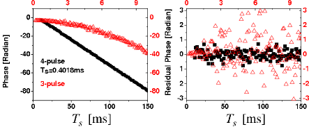
Last, we consider the effect of phase noise in the SW on the sensitivity of our device, induced for example by vibrations of mirrors in the SW path. For $T>>T_{s}$, the standing wave phase variation due to time dependent changes in mirror positions is given by $\varphi_{1,2}$, which is not correlated with $\varphi_{3,4}$. If we specify the SW phase at time $t$ with $\phi(t)$ such that $\varphi_{i}=\phi(T_{i})$, the mirror vibration induced interferometer phase noise is given by $N_{\varphi,{\rm mirror}}(T_{s},T)=\sqrt{2<[\phi(t)-\phi(t+T_{s})]^{2}>_{t}}$, which does not depend on T. This is different from a 3-pulse atom interferometer with mirror-induced phase noise given by $N^{\prime}_{\varphi,{\rm mirror}}(T)=\sqrt{<[\phi(t)-2\phi(t+T/2)+\phi(t+T)]^{2}>_{t}}$, where increases in sensitivity due to increases in interaction time necessarily also result in increases in phase noise. In contrast, in the four pulse scheme considered here $T$ can be increased to improve the sensitivity, while keeping $N_{\varphi,{\rm mirror}}(T_{s})$ unaffected.

This is illustrated in Fig. 6 where we compare the 3-pulse and the 4-pulse interferometer phase readouts under the same noisy environmental conditions. A white noise voltage source is filtered to eliminate frequencies below 100 Hz, then amplified and applied to a piezo-driven mirror in the SW optical path. As shown in Fig. 6, the mirror vibration randomizes the phase of the 3-pulse interferometer for T greater than 5 ms. Under the same conditions, the phase of the 4-pulse interferometer is stable for times longer than 150 ms. In this case the acceleration sensitivity of the 4-pulse interferometer $\delta\varphi/\delta a\sim$1 rad/mm/s² at $T=150$ ms, exceeds that for the 3-pulse case of $\delta\varphi/\delta a\sim$0.4 rad/mm/s² at $T=10$ ms. The insensitivity of the 4-pulse scheme to low-frequency mirror vibrations is a feature of speed-meters, as shown in Eqs. (4), (5) in the semiclassical limit with the phase proportional to the velocity during the interrogation time $T$.

V Summary

We have demonstrated a 4-pulse grating echo interferometer scheme to study the dephasing effects for atoms confined in a magnetic guide. We find linearly reduced dephasing rate at reduced wavepacket displacements, indicating that the matter-wave dephasing is due to very weak potential variation along the waveguide in our setup. We have demonstrated phase stability for an interferometry sequence with total interrogation time exceeding one second. We also show that a four pulse interferometer can provide acceleration measurements with very long integration times that are insensitive to apparatus vibrations, though it is important to note that the sensitivity of the interferometer scheme we describe is compromised by the small wavepacket separations Burke08 .

In the future, such a system could study the quantum stability of wavepackets due to displaced potentials Petitjean et al. (2007) by deliberately introducing time dependent variations in the potential along the waveguide direction  Moore et al. (1995); stability08 . Instead of measuring the mixed-state correlation functions, fidelity-type measurement Petitjean et al. (2007) can be proceeded with sub-recoil cooled atoms occupying a single matter-wave state, where velocity-selective beamsplitting schemes can be applied Wu et al. (2005b); Giltner et al. (1995).