Quantifying bid-ask spreads in the Chinese stock market using limit-order book data

Abstract

The statistical properties of the bid-ask spread of a frequently traded Chinese stock listed on the Shenzhen Stock Exchange are investigated using the limit-order book data. Three different definitions of spread are considered based on the time right before transactions, the time whenever the highest buying price or the lowest selling price changes, and a fixed time interval. The results are qualitatively similar no matter linear prices or logarithmic prices are used. The average spread exhibits evident intraday patterns consisting of a big L-shape in morning transactions and a small L-shape in the afternoon. The distributions of the spread with different definitions decay as power laws. The tail exponents of spreads at transaction level are well within the interval $(2,3)$ and that of average spreads are well in line with the inverse cubic law for different time intervals. Based on the detrended fluctuation analysis, we found the evidence of long memory in the bid-ask spread time series for all three definitions, even after the removal of the intraday pattern. Using the classical box-counting approach for multifractal analysis, we show that the time series of bid-ask spread does not possess multifractal nature.

1 Introduction

The continuous double auction (CDA) is a dominant market mechanism used to store and match orders and to facilitate trading in most modern equity markets Smith-Farmer-Gillemot-Krishnamurthy-2003-QF . In most of the order driven markets, there are two kinds of basic orders, called market orders and limit orders. A market order is submitted to buy or sell a number of shares at the market quote which results in an immediate transaction, while a limit order is placed to buy (or sell) a number of shares below (or above) a given price. All the limit orders that fail to result in an immediate transaction are stored in a queue called limit-order book. Buy limit orders are called bids while sell limit orders are called asks or offers. Best bid price $b(t)$ and best ask (or best offer) price $a(t)$ are the highest buying price and the lowest selling price at any time $t$ in the limit-order book. The best bid (or ask) is called the same best for buy (or sell) orders, while the best ask (or bid) is called the opposite best for buy (or sell) orders. A limit order causes an immediate transaction if the associated limit price penetrates the opposite best price. Such kind of limit orders are called marketable limit orders or effective market orders and other limit orders are termed effective limit orders. In the Chinese stock market, only limit orders were permitted in the placement of orders before July 1, 2006.

It is a dynamic process concerning the limit-order book. Effective limit orders accumulate in the book while effective market orders cause transactions and remove the limit orders according to their price and the time they arrive. Effective limit orders can also be removed by cancelation for a variety of reasons. Unveiling the dynamics of order placement and cancelation will deepen our understanding of the microscopic mechanism of price formation and allow us to reproduce remarkably many key features of common stocks such as the probability distribution of returns Zovko-Farmer-2002-QF ; Gabaix-Gopikrishnan-Plerou-Stanley-2003-Nature ; Bouchaud-Gefen-Potters-Wyart-2004-QF ; Plerou-Gopikrishnan-Gabaix-Stanley-2004-QF ; Farmer-Patelli-Zovko-2005-PNAS ; Malevergne-Pisarenko-Sornette-2005-QF ; Bouchaud-Kockelkoren-Potters-2006-QF ; Mike-Farmer-2007-JEDC .

The difference between best-ask price and best-bid price, $s(t)=a(t)-b(t)$, is the bid-ask spread. Numerous work has been carried out to explore the different components of the bid-ask spread Stoll-1989-JF ; Huang-Stoll-1997-RFS . On the other hand, there are several groups studying the statistical properties of the bid-ask spread time series for different stock markets. Farmer et al. reported that the bid-ask spread defined by $\ln[a(t)]-\ln[b(t)]$ on the London Stock Exchange follows power-law distribution in the tail

$$P(>s)\sim s^{-\zeta}~{},$$ (1)

where the exponent $\zeta=3.03\pm 0.41$ ranging from 2.4 to 3.9 Farmer-Gillemot-Lillo-Mike-Sen-2004-QF ; Mike-Farmer-2007-JEDC , which is well consistent with the inverse cubic law Gopikrishnan-Meyer-Amaral-Stanley-1998-EPJB ; Gabaix-Gopikrishnan-Plerou-Stanley-2003-PA ; Gabaix-Gopikrishnan-Plerou-Stanley-2003-Nature . In addition, Mike and Farmer found that the spread possesses long memory with the Hurst index being $0.75<H<0.85$ Mike-Farmer-2007-JEDC . Plerou et al. adopted the 116 most frequently traded stocks on the New York Stock Exchange over the two-year period 1994-1995 to investigate the coarse-grained bid-ask spread over a time interval $\Delta{t}$ and found that the tail distribution decays as a power law with a mean tail exponent of $\zeta=3.0\pm 0.1$ and the spread after removing the intraday pattern exhibits long memory with $H=0.73\pm 0.01$ Plerou-Gopikrishnan-Stanley-2005-PRE . Qualitatively similar results were found by Cajueiro and Tabak in the Brazilian equity market where the mean tail exponent is $\zeta=2.18$ ranging from 1.18 to 2.97 and the Hurst index is $H=0.68\pm 0.08$ varying from 0.52 to 0.89 Cajueiro-Tabak-2007-PA .

Due to the fast development of the economy of China and the increasing huge capitalization of its stock market, more concerns are attracted to study the emerging Chinese stock market. In order to reduce the market risks and speculation actions, the Chinese stock market adopts $t+1$ trading system, which does not allow traders to sell and buy stocks on the same day, and no market orders were permitted until July 1, 2006, which may however consume the liquidity of the market and cause the spread to show different properties when compared to other stock markets. In this work, we investigated the probability distribution, long memory, and presence of multifractal nature of the bid-ask spread using limit-order book data on the Shenzhen Stock Exchange (SSE) in China.

The rest of this paper is organized as follows. In Sec. 2, we describe in brief the trading rules of the Shenzhen Stock Exchange and the database we adopt. Section 3 introduces three definitions of the bid-ask spread and investigates the intraday pattern in the spread. The cumulative distributions of the spreads for different definitions are discussed in Sec. 4. We show in Sec. 5 the long memory of the spread based on the detrended fluctuation analysis (DFA) quantified by the estimate of the Hurst index. In Sec. 6, we perform multifractal analysis on the bid-ask spread time series. The last section concludes.

2 SSE trading rules and the data set

Our analysis is based on the limit-order book data of a liquid stock listed on the Shenzhen Stock Exchange. SSE was established on December 1, 1990 and has been in operation since July 3, 1991. The securities such as stocks, closed funds, warrants and Lofs can be traded on the Exchange. The Exchange is open for trading from Monday to Friday except the public holidays and other dates as announced by the China Securities Regulatory Commission. With respect to securities auction, opening call auction is held between 9:15 and 9:25 on each trading day, followed by continuous trading from 9:30 to 11:30 and 13:00 to 15:00. The Exchange trading system is closed to orders cancelation during 9:20 to 9:25 and 14:57 to 15:00 of each trading day. Outside these opening hours, unexecuted orders will be removed by the system. During 9:25 to 9:30 of each trading day, the Exchange is open to orders routing from members, but does not process orders or process cancelation of orders.

Auction trading of securities is conducted either as a call auction or a continuous auction. The term “call auction” (from 9:15 to 9:25) refers to the process of one-time centralized matching of buy and sell orders accepted during a specified period in which the single execution price is determined according to the following three principles: (i) the price that generates the greatest trading volume; (ii) the price that allows all the buy orders with higher bid price and all the sell orders with lower offer price to be executed; and (iii) the price that allows either buy orders or sell orders to have all the orders identical to such price to be executed.

The term “continuous auction” (from 9:25 to 11:30 and from 13:00 to 15:00) refers to the process of continuous matching of buy and sell orders on a one-by-one basis and the execution price in a continuous trading is determined according to the following principles: (i) when the best ask price equals to the best bid price, the deal is concluded at such a price; (ii) when the buying price is higher than the best ask price currently available in the central order book, the deal is concluded at the best ask price; and (iii) when the selling price is lower than the best bid price currently available in the central order book, the deal is executed at the best bid price. The orders which are not executed during the opening call auction automatically enter the continuous auction.

The tick size of the quotation price of an order for A shares is RMB 0.01 and that for B shares is HKD 0.01. Orders are matched and executed based on the principle of price-time priority which means priority is given to a higher buy order over a lower buy order and a lower sell order is prioritized over a higher sell order; The order sequence which is arranged according to the time when the Exchange trading system receives the orders determines the priority of trading for the orders with the same prices.

We studied the data from the limit-order book of the stock SZ000001 (Shenzhen Development Bank Co., LTD) in the whole year of 2003. The limit-order book recorded high-frequency data whose time stamps are accurate to 0.01 second. The size of the data set is $3,925,832$, including $12,965$ invalid orders, $122,034$ order submissions and cancelations in the opening call auction, $47,576$ order submissions and cancelations during the cooling period (9:25-9:30), and $3,743,257$ valid events during the continuous auction. In continuous auction, there are $317,015$ cancelations of buy orders and $274,929$ cancelations of sell orders, $889,700$ effective market orders, and $2,261,613$ effective limit orders. Table 1 shows a segment taken from the limit-order book recorded on 2003/07/09. The seven columns stand for order size, limit price, time, best bid, best ask, transaction volume, and buy-sell identifier (which identifies whether a record is a buy order, sell order, or a cancelation). For a cancelation record, the limit price is set to be zero.

Table 1: A segment of the limit-order book

1400	0	9390015	11.33	11.34	0	31
1000	11.48	9390016	11.33	11.34	0	29
400	11.65	9390311	11.33	11.34	0	29
400	0	9390317	11.33	11.34	0	30
1000	11.33	9390365	11.33	11.34	0	26
6000	11.33	9390408	11.33	11.34	6000	23

3 Defining bid-ask spread

The literature concerning the bid-ask spread gives different definitions Farmer-Patelli-Zovko-2005-PNAS ; Mike-Farmer-2007-JEDC ; Stoll-1989-JF ; Huang-Stoll-1997-RFS ; Farmer-Gillemot-Lillo-Mike-Sen-2004-QF ; Plerou-Gopikrishnan-Stanley-2005-PRE ; Cajueiro-Tabak-2007-PA ; Roll-1984-JF ; Daniels-Farmer-Gillemot-Iori-Smith-2003-PRL ; Wyart-Bouchaud-Kockelkoren-Potters-Vettorazzo-2006 . In this section, we discuss three definitions according to sampling time when best bid prices and best ask prices are selected to define the spread. Some definitions are based on the transaction time, while the others are based on the physical time. The latter scheme is actually a coarse-graining of the data within a given time interval.

3.1 Definition I

The first definition of the bid-ask spread used in this work is the absolute or relative difference between the best ask price and the best bid price right before the transaction, that is,

$$s(t)=a(t)-b(t)$$ (2a)

for absolute difference or

$$s(t)=\log_{10}[a(t)]-\log_{10}[b(t)]$$ (2b)

for relative difference. This was used to analyze the stocks on the London Stock Exchange Farmer-Gillemot-Lillo-Mike-Sen-2004-QF ; Mike-Farmer-2007-JEDC . The size of the spread time series is $895,606$.

3.2 Definition II

The best ask price or the best bid price may change due to the removal of all shares at the best price induced by an effective market order, or the placement of an limit order inside the spread, or the cancelation of all limit orders at the best bid/ask price. Hence the bid-ask spread does not always change when a transaction occurs, and it nevertheless changes without transaction. This suggests to introduce an alternative definition of the spread which considers the absolute or relative difference between the best bid price and the best ask price whensoever it changes. The expressions of definition II are the same as those in Eq. (2) except that they have different definitions for the time $t$. The size of the spread time series is $142,913$.

3.3 Definition III

Obviously, the time in the first two definitions are on the basis of “event”. An alternative definition considers the average bid-ask spread over a time interval $\Delta{t}$ Mcinish-Wood-1992-JF . In this definition, the bid-ask spread is the average difference between the best ask the best bid when transactions occur over a fixed time interval Plerou-Gopikrishnan-Stanley-2005-PRE :

$$s(t)=\frac{1}{N}\sum_{i=1}^{N}{s_{i}(t)}~{},~{}~{}~{}s_{i}(t)=a_{i}(t)-b_{i}(t)~{},$$ (3)

where $a_{i}(t)$ and $b_{i}(t)$ are the best ask and bid prices in the time interval $(t-{\Delta}t,t]$, and $N$ is the total number of transaction in the interval and is a function of $t$ and $\Delta{t}$. We use ${\Delta}t=1$, $2$, $3$, $4$, and $5$ minute(s) to calculate the average spreads.

3.4 Intraday pattern

In most modern financial markets, the intraday pattern exists extensively in many financial variables Wood-McInish-Ord-1985-JF ; Harris-1986-JFE ; Admati-Pfleiderer-1988-RFS , including the bid-ask spread Mcinish-Wood-1992-JF . The periodic pattern has significance impact on the detection of long memory in time series Hu-Ivanov-Chen-Carpena-Stanley-2001-PRE . To the best of our knowledge, the investigation of the presence of intraday pattern in the spreads of Chinese stocks is lack.

Figure 1 shows the autocorrelation function $\langle{s(t)s(t+{\ell})}\rangle$ as a function of the time lag $\ell$ for the average bid-ask spread calculated from definition III with linear best bids and asks. We note that the results are very similar when logarithmic prices are adopted in the definition. We see that there are spikes evenly spaced along multiples of 245 min, which is exactly the time span of one trading day. What is interesting is that Fig. 1 indicates that the average spread also possesses half-day periodicity.

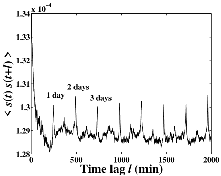
Figure 1: Autocorrelation function $\langle{s(t)s(t+{\ell})}\rangle$ of the average bid-ask spread calculated from definition III with the time interval $\Delta{t}=1$ min. Note that one trading day contains 245 trading minutes in the Chinese stock market.

In order to quantify the intraday pattern, we introduce a variable $A(t)$, which is defined as the average bid-ask spread at time $t$ for all the trading days, that is,

$$A(t)=\frac{1}{M}\sum^{M}_{j=1}{s^{j}(t)}~{},$$ (4)

where $M$ is the number of trading days in the data set and $s^{j}(t)$ is the bid-ask spread at time $t$ of day $j$. The spread $S(t)$ after removing the intraday pattern reads Plerou-Gopikrishnan-Stanley-2005-PRE

$$S(t)=s(t)/A(t)~{}.$$ (5)

Figure 2 illustrates the intraday pattern of the bid-ask spread with ${\Delta}t=1$ minute. The overall plot shows an evident L-shaped pattern, which is consistent with the one-day periodicity shown in the autocorrelation function in Fig. 1. After the opening call auction, the spread $A(t)$ widens rapidly and reaches its maximum 0.0183 at the end of the cooling auction (9:30). Then it decreases sharply in fifteen minutes and becomes flat at a level of $0.0112\pm 0.0008$ afterwards till 11:30. At the begin of continuous auction in the afternoon, $A(t)$ abruptly rises to 0.0133 and drops down to a stable level within about ten minutes which maintains until the closing time 15:00. Therefore, there are two L-shaped patterns each day, which suggests that the wide spread is closely related to the opening of the market. The intraday pattern makes no difference when we use ${\Delta}t=2$, $3$, $4$, and $5$ minutes.

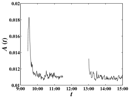
Figure 2: Intraday pattern in the bid-ask spread with $\Delta{t}=1$ min. The spread reaches its maximum at the end of the cooling period at 9:30.

4 Probability distribution

The cumulative distributions of the bid-ask spread of stocks in different stock markets decay as power laws with the tail exponent close to 3 for the major western markets Farmer-Gillemot-Lillo-Mike-Sen-2004-QF ; Plerou-Gopikrishnan-Stanley-2005-PRE ; Mike-Farmer-2007-JEDC and much smaller and more heterogeneous in an emerging market Cajueiro-Tabak-2007-PA . Similar behavior is found in the Chinese stock market. Figure 3 presents the complementary cumulative distribution $P(\geqslant{s})$ of the spreads using definition I and II, where linear prices are used. Since the minimum spread equals to the tick size 0.01, the abscissa is no less than -2 in double logarithmic coordinates and $P(\geqslant 0.01)=1$ for both definitions. The proportion of $s=0.01$ in the first definition is much greater than in the second definition such that the $P(\geqslant{s})$ for the second defintion drops abruptly for small spreads $s$. The two distributions decay as power laws with exponents $\zeta_{\rm{I}}=2.57\pm 0.06$ for definition I and $\zeta_{\rm{II}}=2.30\pm 0.05$ for definition II. When logarithmic prices are utilized, the spreads also follow power-law tail distributions with $\zeta_{\rm{I}}=2.67\pm 0.03$ for definition I and $\zeta_{\rm{II}}=2.42\pm 0.04$ for definition II. Not much difference in the corresponding tail exponents $\zeta_{\rm{I}}$ and $\zeta_{\rm{II}}$ was found for logarithmic and linear prices.

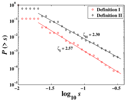
Figure 3: Empirical complementary cumulative distribution of the spreads calculated from definitions I and II using linear prices.

Figure 4 illustrates the complementary cumulative distributions of the average spreads over time interval $\Delta{t}=1$, $2$, $3$, $4$, and $5$ minute(s) calculated from definition III with linear prices. The average spreads have power-law tails with the exponents equal to $\zeta_{\rm{III},1}=2.99\pm 0.04$, $\zeta_{\rm{III},2}=3.00\pm 0.04$, $\zeta_{\rm{III},3}=3.00\pm 0.05$, $\zeta_{\rm{III},4}=2.95\pm 0.05$, and $\zeta_{\rm{III},5}=2.97\pm 0.06$. Similarly, for logarithmic prices, we find similar power-law tail distributions with $\zeta_{\rm{III},1}=3.07\pm 0.06$, $\zeta_{\rm{III},2}=2.95\pm 0.05$, $\zeta_{\rm{III},3}=3.00\pm 0.04$, $\zeta_{\rm{III},4}=2.97\pm 0.07$, and $\zeta_{\rm{III},5}=2.98\pm 0.07$. We find that all the tail exponents $\zeta_{{\rm{III}},\Delta{t}}$ for both linear and logarithmic prices are very close to three and are independent to the time interval $\delta{t}$, showing a nice inverse cubic law. This is well in agreement with the results in the NYSE case for $\Delta{t}=15$, $30$, and $60$ min Plerou-Gopikrishnan-Stanley-2005-PRE .

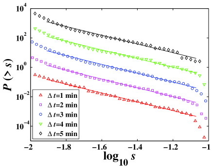
Figure 4: Empirical complementary cumulative distributions of the average spreads calculated from definition III with time intervals ${\Delta}t=1$, $2$, $3$, $4$, and $5$ min using linear prices. The markers represent the real data and the solid lines are the best fits in the scaling ranges. The curves with $\Delta{t}>1$ has been translated vertically for clarity.

There are also significant discrepancies. Comparing the cumulative distributions in Fig. 4 and that on the NYSE Plerou-Gopikrishnan-Stanley-2005-PRE , significant differences are observed. The distribution of the spreads on the SSE decays much faster than that on the NYSE for small spreads. In other words, the proportion of small spreads is much larger on China’s SSE. Possible causes include the absence of market orders, no short positions, the maximum percentage of fluctuation (10%) in each day, and the $t+1$ trading mechanism in the Chinese stock markets on the one hand and the hybrid trading system containing both specialists and limit-order traders in the NYSE on the other hand. The exact cause is not clear for the time being, which can however be tested when new data are available after the introduction of market orders in July 1, 2006. Moreover, the PDF’s in SSE drop abruptly after the power-law parts for the largest spreads, which is not observed in the NYSE case Plerou-Gopikrishnan-Stanley-2005-PRE .

5 Long memory

Another important issue about financial time series is the presence of long memory, which can be characterized by its Hurst index $H$. If $H$ is significantly larger than $0.5$ the time series is viewed to possess long memory. Long memory can be defined equivalently through autocorrelation function $C(\ell)\sim\ell^{-{\gamma}}$ and the power spectrum $p(\omega)\sim\omega^{-\eta}$, where the autocorrelation exponent ${\gamma}$ is related to the Hurst index $H$ by $\gamma=2-2H$ Kantelhardt-Bunde-Rego-Havlin-Bunde-2001-PA ; Maraun-Rust-Timmer-2004-NPG , and the power spectrum exponent $\eta$ is given by $\eta=2H-1$ Talkner-Weber-2000-PRE ; Heneghan-McDarby-2000-PRE .

There are many methods proposed for estimating the Hurst index such as the rescaled range analysis (RSA) Hurst-1951-TASCE ; Mandelbrot-Ness-1968-SIAMR ; Mandelbrot-Wallis-1969a-WRR ; Mandelbrot-Wallis-1969b-WRR ; Mandelbrot-Wallis-1969c-WRR ; Mandelbrot-Wallis-1969d-WRR , fluctuation analysis (FA) Peng-Buldyrev-Goldberger-Havlin-Sciortino-Simons-Stanley-1992-Nature , detrended fluctuation analysis (DFA) Peng-Buldyrev-Havlin-Simons-Stanley-Goldberger-1994-PRE ; Hu-Ivanov-Chen-Carpena-Stanley-2001-PRE ; Kantelhardt-Bunde-Rego-Havlin-Bunde-2001-PA , wavelet transform module maxima (WTMM) method Holschneider-1988-JSP ; Muzy-Bacry-Arneodo-1991-PRL ; Muzy-Bacry-Arneodo-1993-JSP ; Muzy-Bacry-Arneodo-1993-PRE ; Muzy-Bacry-Arneodo-1994-IJBC , detrended moving average (DMA) Alessio-Carbone-Castelli-Frappietro-2002-EPJB ; Carbone-Castelli-Stanley-2004-PA ; Carbone-Castelli-Stanley-2004-PRE ; Alvarez-Ramirez-Rodriguez-Echeverria-2005-PA ; Xu-Ivanov-Hu-Chen-Carbone-Stanley-2005-PRE , to list a few. We adopt the detrended fluctuation analysis.

The method of detrended fluctuation analysis is widely used for its easy implementation and robust estimation even for a short time series Taqqu-Teverovsky-Willinger-1995-Fractals ; Montanari-Taqqu-Teverovsky-1999-MCM ; Heneghan-McDarby-2000-PRE ; Audit-Bacry-Muzy-Arneodo-2002-IEEEtit . The idea of DFA was invented originally to investigate the long-range dependence in coding and noncoding DNA nucleotides sequencePeng-Buldyrev-Havlin-Simons-Stanley-Goldberger-1994-PRE and then applied to various fields including finance. The method of DFA consists of the following steps.

Step 1: Consider a time series $x(t)$, $t=1,2,\cdots,N$. We first construct the cumulative sum

$$u(t)=\sum_{i=1}^{t}{x(i)},~{}~{}t=1,2,\cdots,N~{}.$$ (6)

Step 2: Divide the series $u(t)$ into $N_{\ell}$ disjoint segments with the same length $\ell$, where $N_{\ell}=[N/\ell]$. Each segment can be denoted as $u_{v}$ such that $u_{v}(i)=u(l+i)$ for $1\leqslant{i}\leqslant{\ell}$, and $l=(v-1)\ell$. The trend of $u_{v}$ in each segment can be determined by fitting it with a linear polynomial function $\widetilde{u}_{v}$. Quadratic, cubic or higher order polynomials can also be used in the fitting procedure while the simplest function could be linear. In this work, we adopted the linear polynomial function to represent the trend in each segment with the form:

$$\widetilde{u}_{v}(i)=ai+b~{},$$ (7)

where $a$ and $b$ are free parameters to be determined by the least squares fitting method and $1\leqslant{i}\leqslant\ell$.

Step 3: We can then obtain the residual matrix $\epsilon_{v}$ in each segment through:

$$\epsilon_{v}(i)=u_{v}(i)-\widetilde{u}_{v}(i)~{},$$ (8)

where $1\leqslant{i}\leqslant{\ell}$. The detrended fluctuation function $F(v,\ell)$ of the each segment is defined via the sample variance of the residual matrix $\epsilon_{v}$ as follows:

$$F^{2}(v,\ell)=\frac{1}{\ell}\sum_{i=1}^{\ell}[\epsilon_{v}(i)]^{2}~{}.$$ (9)

Note that the mean of the residual is zero due to the detrending procedure.

Step 4: Calculate the overall detrended fluctuation function $F(\ell)$, that is,

$$F^{2}(\ell)=\frac{1}{N_{\ell}}\sum_{v=1}^{N_{\ell}}F^{2}(v,\ell)~{}.$$ (10)

Step 5: Varying the value of $\ell$, we can determine the scaling relation between the detrended fluctuation function $F(\ell)$ and the size scale $\ell$, which reads

$$F(\ell)\sim\ell^{H}~{},$$ (11)

where $H$ is the Hurst index of the time series Taqqu-Teverovsky-Willinger-1995-Fractals ; Kantelhardt-Bunde-Rego-Havlin-Bunde-2001-PA .

Figure 5 plots the detrended fluctuation function $F(\ell)$ of the bid-ask spreads from different definitions using linear prices. The bottom $F(\ell)$ curve is for the average spread after removing the intraday pattern. All the curves show evident power-law scaling with the Hurst indexes $H_{\rm{I}}=0.91\pm 0.01$ for definition I, $H_{\rm{II}}=0.92\pm 0.01$ for definition II, $H_{\rm{III}}=0.75\pm 0.01$ for definition III, and $H_{\rm{III}}=0.77\pm 0.01$ for definition without intraday pattern, respectively. Quite similar results are obtain for logarithmic prices where $H_{\rm{I}}=0.89\pm 0.01$ for definition I, $H_{\rm{II}}=0.91\pm 0.01$ for definition II, $H_{\rm{III}}=0.77\pm 0.01$ for definition III, and $H_{\rm{III}}=0.76\pm 0.01$ for definition III without intraday pattern. The two Hurst indexes for definitions I and II are higher than their counterparts on the London Stock Exchange where “even time” is adopted Mike-Farmer-2007-JEDC . It is interesting to note that the presence of intraday pattern does not introduce distinguishable difference in the Hurst index and the two indexes for definition III are also very close to those of average spreads in the Brazilian stock market and on the New York Stock Exchange where real time is used Plerou-Gopikrishnan-Stanley-2005-PRE ; Cajueiro-Tabak-2007-PA . Due to the large number of data used in the analysis, we argue that the bid-ask spreads investigated exhibit significant long memory.

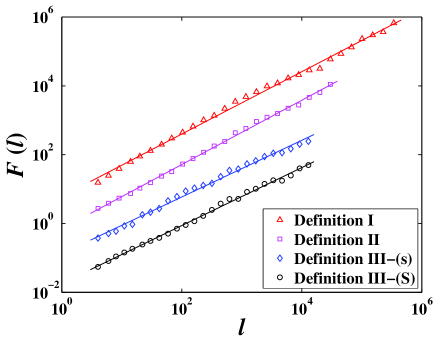
Figure 5: Detrended fluctuation function $F(\ell)$ for the spreads obtained from three definition with linear prices. The curves have been shifted vertically for clarity.

6 Multifractal analysis

In this section, we investigate whether the time series of bid-ask spread obtained from definition III possesses multifractal nature. The classical box-counting algorithm for multifractal analysis is utilized and described below Halsey-Jensen-Kadanoff-Procaccia-Shraiman-1986-PRA .

Consider the spread time series $S(t)$, $t=1,2,\cdots,N$. First, we divide the series $S(t)$ into $N_{\ell}$ disjoint segments with the same length $\ell$, where $N_{\ell}=[N/\ell]$. Each segment can be denoted as $S_{v}$ such that $S_{v}(i)=S(l+i)$ for $1\leqslant{i}\leqslant{\ell}$, and $l=(v-1)\ell$. The sum of $S_{v}$ in each segment is calculated as follows,

$$\Gamma(v,\ell)=\sum_{i=1}^{\ell}{S_{v}(i)},~{}~{}v=1,2,\cdots,N_{\ell}~{}.$$ (12)

We can then calculate the $q$th order partition function $\Gamma(q;\ell)$ as follows,

$$\Gamma(q;\ell)=\sum_{v=1}^{N_{\ell}}[\Gamma(v,\ell)]^{q}~{}.$$ (13)

Varying the value of $\ell$, we can determine the scaling relation between the partition function $\Gamma(q;\ell)$ and the time scale $\ell$, which reads

$$\Gamma(q;\ell)\sim\ell^{\tau(q)}~{}.$$ (14)

Figure 6 illustrates the power-law scaling dependence of the partition function $\Gamma(q;\ell)$ of the bid-ask spreads after removing the intraday pattern in definition III for different values of $q$, where both linear prices and logarithmic prices are investigated. The continuous lines are the best linear fits to the data sets. The collapse of the data points on the linear lines indicates evident power-law scaling between $\Gamma(q;\ell)$ and $\ell$. The slopes $\tau(q)$ of the fitted lines are $\tau(-4)=-5.02\pm 0.01$, $\tau(-2)=-3.01\pm 0.01$, $\tau(0)=-1.01\pm 0.01$, $\tau(2)=0.99\pm 0.01$, and $\tau(4)=2.98\pm 0.01$ for logarithmic prices and $\tau(-4)=-5.02\pm 0.01$, $\tau(-2)=-3.01\pm 0.01$, $\tau(0)=-1.01\pm 0.01$, $\tau(2)=0.99\pm 0.01$, and $\tau(4)=2.98\pm 0.01$ for linear prices. We notice a nice relation $\tau(q)=q-1$.

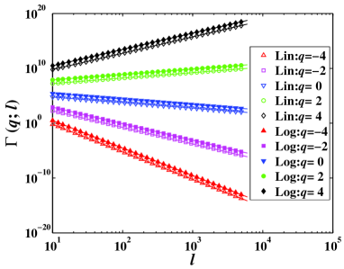
Figure 6: Log-log plots of the partition function $\Gamma(q;\ell)$ of the bid-ask spreads calculated from definition III with the intraday pattern removed for five different values of $q$. Both linear and logarithmic prices are investigated (shown in the legend). The markers stand for the results calculated from the real data and the continuous lines are the best fits. The plots for $q=-2,0,2$, and $4$ are shifted upwards for clarity.

Quantitatively similar results are obtained when the intraday pattern is not removed. The scaling exponents are $\tau(-4)=-5.03\pm 0.01$, $\tau(-2)=-3.01\pm 0.01$, $\tau(0)=-1.01\pm 0.01$, $\tau(2)=0.99\pm 0.01$, and $\tau(4)=2.96\pm 0.01$ for logarithmic prices and $\tau(-4)=-5.03\pm 0.01$, $\tau(-2)=-3.02\pm 0.01$, $\tau(0)=-1.01\pm 0.01$, $\tau(2)=0.99\pm 0.01$, and $\tau(4)=2.97\pm 0.01$ for linear prices. Again, we observe that $\tau(q)=q-1$.

In the standard multifractal formalism based on partition function, the multifractal nature is characterized by the scaling exponents $\tau(q)$. It is easy to obtain the generalized dimensions $D_{q}={\tau}(q)/(q-1)$ Grassberger-1983-PLA ; Hentschel-Procaccia-1983-PD ; Grassberger-Procaccia-1983-PD and the singularity strength function $\alpha(q)$, the multifractal spectrum $f(\alpha)$ via the Legendre transform Halsey-Jensen-Kadanoff-Procaccia-Shraiman-1986-PRA : $\alpha(q)={\rm d}{\tau}(q)/{\rm d}q$ and $f(q)=q{\alpha}-{\tau}(q)$.

Figure 7 shows the multifractal spectrum $f(\alpha)$ and the scaling function $\tau(q)$ in the inset for linear and logarithmic prices. One finds that the two $\tau(q)$ curves are linear and $\tau(q)=q-1$, which is the hallmark of the presence of monofractality, not multifractality. The strength of the multifractality can be characterized by the span of singularity $\Delta\alpha=\alpha_{\max}-\alpha_{\min}$. If $\Delta\alpha$ is close to zero, the measure is almost monofractal. The maximum and minimum of $\alpha$ can be reached when $q\to\pm\infty$, which can not be achieved in real applications. However, $\Delta\alpha$ can be approximated with great precision with mediate values of $q$. The small value of $\Delta\alpha$ shown in Fig. 7 indicates a very narrow spectrum of singularity. Indeed, one sees that $f(\alpha)\approx 1$ and $\alpha\approx 1$ for all values of $q$. We thus conclude that there is no multifractal nature in the bid-ask spread investigated.

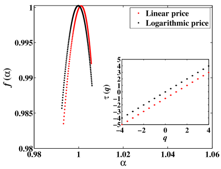
Figure 7: Multifractal function $f({\alpha})$ of the spreads in definition III with the intraday pattern removed. Inset: Scaling exponents ${\tau}(q)$ of partition functions as a function of $q$. For clarity, the $\tau(q)$ curve for logarithmic price is shifted upwards by 1.

7 Conclusions

The bid-ask spread defined by the difference of the best ask price and the best bid price is considered as the benchmark of the transaction cost and a measure of the market liquidity. In this paper, we have carried out empirical investigations on the statistical properties of the bid-ask spread using the limit-order book data of a stock SZ000001 (Shenzhen Development Bank Co., LTD) traded on the Shenzhen Stock Exchange within the whole year of 2003. Three different definitions of spread are considered based on event time at transaction level and on fixed interval of real time.

The distributions of spreads at transaction level decay as power laws with tail exponents well below 3. In contrast the average spread in real time fulfils the inverse cubic law for different time intervals $\Delta{t}=1$, $2$, $3$, $4$, and $5$ min. We have performed the detrended fluctuation analysis on the spread and found that the spread time series exhibits evident long-memory, which is in agreement with other stock markets. However, an analysis using the classic textbook box-counting algorithm does not provide evidence for the presence of multifractality in the spread time series. To the best of our knowledge, this is the first time to check the presence of multifractality in the spread.

Our analysis raises an intriguing open question that is not fully addressed. We have found that the spread possesses a well-established intraday pattern composed by a large L-shape and a small L-shape separated by the noon closing of the Chinese stock market. This feature will help to understand the cause of the wide spread at the opening of the market, which deserves further investigation.

- (1) E. Smith et al., Quant. Finance 3 (2003) 481.
- (2) I. Zovko and J.D. Farmer, Quant. Finance 2 (2002) 387.
- (3) X. Gabaix et al., Nature 423 (2003) 267.
- (4) J.P. Bouchaud et al., Quant. Finance 4 (2004) 176.
- (5) V. Plerou et al., Quant. Finance 4 (2004) C11.
- (6) J.D. Farmer, P. Patelli and I.I. Zovko, Proc. Natl. Acad. Sci. USA 102 (2005) 2254.
- (7) Y. Malevergne, V. Pisarenko and D. Sornette, Quant. Finance 5 (2005) 379.
- (8) J.P. Bouchaud, J. Kockelkoren and M. Potters, Quant. Finance 6 (2006) 115.
- (9) S. Mike and J.D. Farmer, J. Econ. Dyn. Control (2007) forthcoming.
- (10) H.R. Stoll, J. Finance 44 (1989) 115.
- (11) R.D. Huang and H.R. Stoll, Rev. Fin. Stud. 10 (1997) 995.
- (12) J.D. Farmer et al., Quant. Finance 4 (2004) 383.
- (13) P. Gopikrishnan et al., Eur. Phys. J. B 3 (1998) 139.
- (14) X. Gabaix et al., Physica A 324 (2003) 1.
- (15) V. Plerou, P. Gopikrishnan and S. H.E., Phys. Rev. E 71 (2005) 046131.
- (16) D.O. Cajueiro and B.M. Tabak, Physica A 373 (2007) 627.
- (17) R. Roll, J. Finance 39 (1984) 1127.
- (18) M.G. Daniels et al., Phys. Rev. Lett. 90 (2003) 108102.
- (19) M. Wyart et al., Relation between bid-ask spread, impact and volatility in double auction markets, physics/0603084, 2006.
- (20) T.H. Mcinish and R.A. Wood, J. Finance 47 (1992) 753.
- (21) R.A. Wood, T.H. McInish and J.K. Ord, J. Finance 40 (1985) 723.
- (22) L. Harris, J. Fin. Econ. 16 (1986) 99.
- (23) A.R. Admati and P. Pfleiderer, Rev. Fin. Stud. 1 (1988) 3.
- (24) K. Hu et al., Phys. Rev. E 64 (2001) 011114.
- (25) J.W. Kantelhardt et al., Physica A 316 (2001) 441.
- (26) D. Maraun, H.W. Rust and J. Timmer, Nonlin. Processes Geophys. 11 (2004) 495.
- (27) P. Talkner and R.O. Weber, Phys. Rev. E 62 (2000) 150.
- (28) C. Heneghan and G. McDarby, Phys. Rev. E 62 (2000) 6103.
- (29) H.E. Hurst, Transactions of the American Society of Civil Engineers 116 (1951) 770.
- (30) B.B. Mandelbrot and J.W. Van Ness, SIAM Rev. 10 (1968) 422.
- (31) B.B. Mandelbrot and J.R. Wallis, Water Resour. Res. 5 (1969) 228.
- (32) B.B. Mandelbrot and J.R. Wallis, Water Resour. Res. 5 (1969) 242.
- (33) B.B. Mandelbrot and J.R. Wallis, Water Resour. Res. 5 (1969) 260.
- (34) B.B. Mandelbrot and J.R. Wallis, Water Resour. Res. 5 (1969) 967.
- (35) C.K. Peng et al., Nature 356 (1992) 168.
- (36) C.K. Peng et al., Phys. Rev. E 49 (1994) 1685.
- (37) M. Holschneider, J. Stat. Phys. 50 (1988) 953.
- (38) J.F. Muzy, E. Bacry and A. Arnéodo, Phys. Rev. Lett. 67 (1991) 3515.
- (39) J.F. Muzy, E. Bacry and A. Arnéodo, J. Stat. Phys. 70 (1993) 635.
- (40) J.F. Muzy, E. Bacry and A. Arnéodo, Phys. Rev. E 47 (1993) 875.
- (41) J.F. Muzy, E. Bacry and A. Arnéodo, Int. J. Bifur. Chaos 4 (1994) 245.
- (42) E. Alessio et al., Eur. Phys. J. B 27 (2002) 197.
- (43) A. Carbone, G. Castelli and H.E. Stanley, Physica A 344 (2004) 267.
- (44) A. Carbone, G. Castelli and H.E. Stanley, Phys. Rev. E 69 (2004) 026105.
- (45) J. Alvarez-Ramirez, E. Rodriguez and J.C. Echeverría, Physica A 354 (2005) 199.
- (46) L.M. Xu et al., Phys. Rev. E 71 (2005) 051101.
- (47) M. Taqqu, V. Teverovsky and W. Willinger, Fractals 3 (1995) 785.
- (48) A. Montanari, M.S. Taqqu and V. Teverovsky, Math. Comput. Modell. 29 (1999) 217.
- (49) B. Audit et al., IEEE Trans. Info. Theory 48 (2002) 2938.
- (50) T.C. Halsey et al., Phys. Rev. A 33 (1986) 1141.
- (51) P. Grassberger, Physics Letters A 97 (1983) 227.
- (52) H.G.E. Hentschel and I. Procaccia, Physica D 8 (1983) 435.
- (53) P. Grassberger and I. Procaccia, Physica D 9 (1983) 189.