Harris sheet solution for magnetized quantum plasmas

Abstract

We construct an infinite family of one-dimensional equilibrium solutions for purely magnetized quantum plasmas described by the quantum hydrodynamic model. The equilibria depends on the solution of a third-order ordinary differential equation, which is written in terms of two free functions. One of these free functions is associated to the magnetic field configuration, while the other is specified by an equation of state. The case of a Harris sheet type magnetic field, together with an isothermal distribution, is treated in detail. In contrast to the classical Harris sheet solution, the quantum case exhibits an oscillatory pattern for the density.

1 Introduction

Quantum plasmas have attracted renewed attention in the last years, due e.g. to the relevance of quantum effects in ultra-small semiconductor devices [1], dense plasmas [2] and very intense laser plasmas [3]. The most recent developments in collective effects in quantum plasmas comprises wave propagation in dusty plasmas [4]-[9], soliton and vortex solutions [10, 11], shielding effects [12, 13], modulational instabilities [14] and spin effects [15]. Most of these works have been made using the hydrodynamic model for quantum plasmas [16]-[20], in contrast to more traditional approaches based on kinetic descriptions [21]. Microscopic descriptions like coupled Schrödinger equations or Wigner function approaches are more expensive, both numerically and analytically, specially if magnetic fields are allowed. For a general review on the available quantum plasma models, see [22].

The electrostatic fluid model for quantum plasmas have been recently extended to incorporate magnetic fields [23]. The new quantum hydrodynamic model was derived taking the first two moments of the electromagnetic Wigner equation, which is the quantum counterpart of the corresponding Vlasov equation, and assuming a closure condition $p=p(n)$. In other words, the procedure is formally the same as for classical plasma fluid descriptions, while now the starting point is the Wigner-Maxwell and not the Vlasov-Maxwell system. The electromagnetic quantum fluid model has been already used for the analysis of shear Alfvén modes in ultra-cold quantum magnetoplasmas [24], the description of drift modes in nonuniform quantum magnetoplasmas [25] and of shear electromagnetic waves in electron-positron plasmas [26]. Instead of the discussion of wave propagation in quantum plasmas, the aim of this letter is the analysis of some simple quantum magnetostatic equilibria resembling the well known Harris profile for classical plasma [27].

2 Quantum magnetoplasma equilibria

For a one-component quantum plasma, the electromagnetic quantum fluid equations reads [23]

$$\frac{\partial n}{\partial t}+\nabla\cdot(n{\bf u}) = 0\,,$$ (1)

$$\frac{\partial{\bf u}}{\partial t}+{\bf u}\cdot\nabla{\bf u} = -\frac{1}{mn}\nabla\,p-\frac{e}{m}({\bf E}+{\bf u}\times{\bf B})$$ (2)

$$+ \frac{\hbar^{2}}{2m^{2}}\nabla\left(\frac{\nabla^{2}\sqrt{n}}{\sqrt{n}}\right)\,.$$

All the symbols in eqs. (1-2) have their conventional meaning and the system is supplemented by Maxwell equations. Only electrons are considered, the ions being described by a convenient immobile background. Notice the extra dispersive term, proportional to $\hbar^{2}$, at the moment transport equation. This Bohm potential term has profound consequences on the structure of the equilibrium solutions, as we shall see in the following.

Specifically, consider a purely magnetic one-dimensional class of time-independent solutions characterized by zero electric field and

$${\bf B} = B_{y}(x)\hat{y}+B_{z}(x)\hat{z}\,,$$

$$n = n(x)\,,$$ (3)

$${\bf u} = u_{y}(x)\hat{y}+u_{z}(x)\hat{z}\,,$$

$$p = p(n)\,.$$

The magnetic field can be given in terms of a vector potential ${\bf A}=A_{y}(x)\hat{y}+A_{z}(x)\hat{z}$, so that $B_{y}=-dA_{z}/dx$ and $B_{z}=dA_{y}/dx$. Notice that the fluid model is suitable for the search for static quantum equilibria since the kinetic (Wigner) equation is not satisfied by arbitrary functions of the invariants of motion as for Vlasov plasmas. Therefore we are not allowed to use Jeans theorem for the construction of equilibria.

Neutrality is enforced by an appropriate immobile ionic background described by an ionic density $n_{i}(x)$. Therefore, Poisson’s equation can be ignored. Now inserting the form (3) into Ampère’s law and the quantum fluid equations gives

$$\frac{d^{2}A_{y}}{dx^{2}} = e\mu_{0}nu_{y}\,,$$ (4)

$$\frac{d^{2}A_{z}}{dx^{2}} = e\mu_{0}nu_{z}\,,$$ (5)

$$\frac{dp}{dx} = -en(u_{y}\frac{dA_{y}}{dx}+u_{z}\frac{dA_{z}}{dx})$$ (6)

$$+ \frac{\hbar^{2}n}{2m}\frac{d}{dx}\left(\frac{d^{2}\sqrt{n}/dx^{2}}{\sqrt{n}}\right)\,.$$

As in the classical situation [28], it is useful to restrict to the cases where the magnetic field is indirectly defined through a pseudo-potential $V=V(A_{y},A_{z})$ for which

$$nu_{y}=-\frac{1}{e\mu_{0}}\frac{\partial V}{\partial A_{y}}\,,$$ (7)

$$\quad nu_{z}=-\frac{1}{e\mu_{0}}\frac{\partial V}{\partial A_{z}}\,,$$ (8)

so that (4-5) is transformed into a two-dimensional autonomous Hamiltonian system,

$$\frac{d^{2}A_{y}}{dx^{2}} = -\frac{\partial V}{\partial A_{y}}\,,$$ (9)

$$\frac{d^{2}A_{z}}{dx^{2}} = -\frac{\partial V}{\partial A_{z}}\,.$$ (10)

In this system, $x$ plays the rôle of time, while the components of the vector potential play the rôle of spatial coordinates. After specifying the pseudo-potential $V$ and solving eqs. (9-10), we regain the magnetic field using ${\bf B}=\nabla\times{\bf A}$. The current then follows from eqs. (7-8).

The choice expressed at eqs. (7-8) imposes a restriction on the classes of equilibria, since not all density and velocity fields can be cast in this potential form. However, introducing the pseudo-potential $V$ has at least two advantages. First, we can learn from Hamiltonian dynamics how to design specific pseudo-potentials $V$ in order to obtain special classes of magnetic fields. For instance, periodic magnetic fields can be easily obtained from well known potentials associated to periodic solutions. Second, the formalism becomes more compact in terms of the function $V$.

In terms of $V$, the balance eq. (6) reads

$$\frac{d}{dx}\left(p-\frac{V}{\mu_{0}}\right)=\frac{\hbar^{2}n}{2m}\frac{d}{dx}\left(\frac{d^{2}\sqrt{n}/dx^{2}}{\sqrt{n}}\right)\,.$$ (11)

It can be shown that, apart from an irrelevant numerical constant, the pseudo-potential $V$ is directly related to magnetic pressure, $V=-|{\bf B}|^{2}/2$, showing that the left-hand side of eq. (11) refers to the usual (classical) pressure balance equation. The right-hand side, however, has a pure quantum nature. Not only there must be a balance between kinetic and magnetic pressures, since the quantum pressure arising from the Bohm potential term has to be taken into account. This quantum pressure manifests e.g. in the dispersion of wave-packets in standard quantum mechanics. In plasmas, the quantum pressure is responsible for subtle effects like in the case of the quantum two-stream instability, where the instability is magnified for small wave-numbers and suppressed for large wave-numbers [16, 20].

In the quantum case where $\hbar\neq 0$, eq. (11) is a third-order ODE for the density. It is useful to express this equation in terms of a variable $a=\sqrt{n}$. Taking into account the equation of state $p=p(n)$ and defining a new function $\tilde{V}(x)=V(A_{y}(x),A_{z}(x))$, we get

$$aa^{\prime\prime\prime}-a^{\prime}a^{\prime\prime}+f(a)a^{\prime}+g(x)=0\,,$$ (12)

where the prime denotes differentiation with respect to $x$ and we have introduced the quantities

$$f(a) = -\frac{4ma}{\hbar^{2}}\frac{dp}{dn}(n=a^{2})\,,$$ (13)

$$g(x) = \frac{2m}{\mu_{0}\hbar^{2}}\frac{d\tilde{V}}{dx}\,.$$ (14)

The strategy to derive the solutions is now clear. Choosing a pseudo-potential $V(A_{y},A_{z})$ and then solving the Hamiltonian system (9-10) for the vector potential, we determine simultaneously the magnetic field and $\tilde{V}$. Quantum effects manifests in the equation for the density, eq. (12), which also deserves the function of state $p=p(n)$.

Another legitimate interpretation of the balance equation (12) is to first specify the particle density $n$ and the magnetic pressure $-V/\mu_{0}$ and then solving for the kinetic pressure. This would give an equation of state with a quantum correction. However, in most applications, one supposes a certain equation of state and then proceeds to the calculation of the density and velocity fields. This will be our preferred approach in what follows. In the next section, we consider in detail the case of Harris sheet magnetic fields.

3 Quantum Harris sheet

Exactly as for the classical Harris solution, suppose a isothermal plasma, $p=n\kappa_{B}T$, and a pseudo-potential function

$$V=\frac{B_{\infty}^{2}}{2}\exp(\frac{2A_{z}}{B_{\infty}L})\,,$$ (15)

where $L$ is a characteristic length and $B_{\infty}$ is a (constant) magnetic field reference value. The Hamiltonian system (9-10) is then

$$\frac{d^{2}A_{y}}{dx^{2}}=0\,,\quad\frac{d^{2}A_{z}}{dx^{2}}=-\frac{B_{\infty}}{L}\exp(\frac{2A_{z}}{B_{\infty}L})\,.$$ (16)

If we further take the boundary conditions $A_{z}(x=0)=(dA_{z}/dx)(x=0)=0$, we easily solve (16) to get

$$A_{y}=A_{y0}+B_{0}x\,,\quad A_{z}=-B_{\infty}L\,\ln\cosh(x/L)\,,$$ (17)

where $A_{y0}$ and $B_{0}$ are integration constants. The magnetic field following from this vector potential characterizes the well-known Harris sheet solution,

$$B_{y}=B_{\infty}\tanh(x/L)\,,\quad B_{z}=B_{0}\,,$$ (18)

also allowing for a superimposed homogeneous magnetic field.

In addition, the velocity field follows from (4-5),

$$u_{y}=0\,,\quad u_{z}=\frac{B_{\infty}}{e\mu_{0}nL}\sec\!{\rm h}^{2}(\frac{x}{L})\,.$$ (19)

Notice that any departure from the classical density solution would imply further changes in the velocity field.

To derive the density we have to solve the third-order ODE eq. (12), constructed in terms of the functions $f(a)$ and $g(x)$ at (13-14). Using the isothermal equation of state, the form (15) for the pseudo-potential $V$ and the Harris sheet solution, we get

$$f(a) = -\frac{4m\kappa_{B}T}{\hbar^{2}}\,a\,,$$ (20)

$$g(x) = -\frac{mB_{\infty}^{2}}{\mu_{0}\hbar^{2}L}\sec\!{\rm h}^{2}(\frac{x}{L})\tanh(\frac{x}{L})\,.$$ (21)

Adopting the dimensionless variables

$$\alpha=a/\sqrt{n_{0}}\,,\quad X=x/L\,,$$ (22)

where $n_{0}$ is some ambient density such that

$$n_{0}\kappa_{B}T=\frac{B_{\infty}^{2}}{4\mu_{0}}\,,$$ (23)

eq. (8) is finally expressed as

$$\alpha\frac{d^{3}\alpha}{dX^{3}}-\frac{d\alpha}{dX}\frac{d^{2}\alpha}{dX^{2}}-\frac{\alpha}{H^{2}}\,\frac{d\alpha}{dX}=\frac{1}{H^{2}}\,\sec\!{\rm h}^{2}X\tanh\,X\,,$$ (24)

in terms of a new dimensionless parameter

$$H=\frac{\hbar}{mV_{a}L}\,,$$ (25)

where $V_{a}=B_{\infty}/(\mu_{0}mn_{0})^{1/2}$ is the Alfvén velocity.

The parameter $H$ is a measure of the relevance of the quantum effects. It is essentially the ratio of the scaled Planck constant $\hbar$ to the action of a particle of mass $m$ travelling with the Alfvén velocity and confined in a length $L$ related to the thickness of the sheet. The larger the ambient density $n_{0}$ and the smaller the characteristic length $L$ or the characteristic magnetic field $B_{\infty}$, the larger are the quantum effects.

In order to understand the rôle of the quantum terms, we may investigate (24) with

$$\alpha(X=0)=1\,,\quad\frac{d\alpha}{dX}(X=0)=0\,,\quad\frac{d^{2}\alpha}{dX^{2}}(X=0)=-1\,,$$ (26)

which reproduces the boundary conditions for the classical Harris sheet, when $\alpha=\sec\!{\rm h}X$. With the choice (26), eq. (24) integrated once gives

$$\alpha\frac{d^{2}\alpha}{dX^{2}}-\left(\frac{d\alpha}{dX}\right)^{2}+1=\frac{1}{2H^{2}}\,\left(\alpha^{2}-\sec\!{\rm h}^{2}X\right)\,.$$ (27)

In the ultra-quantum limit $H\rightarrow\infty$, the left-hand side of (27) vanishes. In this situation and using the prescribed boundary conditions, the solution is

$$\alpha=\cos X\,.$$ (28)

This imply a qualitative change (from localized to oscillatory) on the solution due to quantum effects. In order to further investigate this tendency, we show the numerical solution for (27) with the appropriate boundary conditions for a few values of $H$. This is shown in the figs. 1 and 2, where increasingly oscillatory solutions are shown, according to $H=1$ or $H=5$ respectively. On the opposite case, (27) shows that when $H\rightarrow 0$ we regain the classical Harris solution, $\alpha=\sec\!{\rm h}X$.

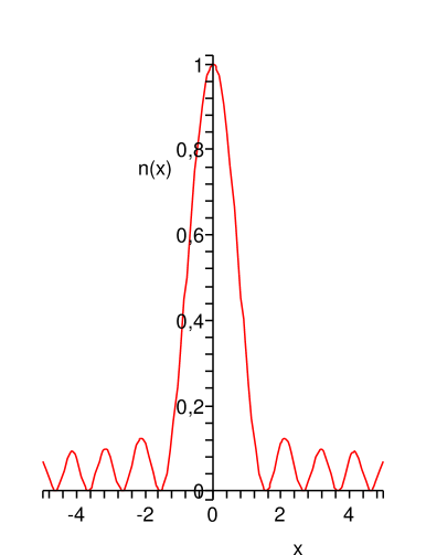
Figure 1: Density oscillations for $H=1$. Parameters: $n_{0}=L=1$.

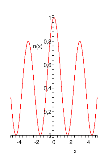
Figure 2: Density oscillations for $H=5$. Parameters: $n_{0}=L=1$.

Another interesting possibility is an equation of state for an ultra-cold Fermi gas,

$$p=\frac{2\kappa_{B}T_{F}}{5n_{0}^{2/3}}\,n^{5/3}\,,$$ (29)

where $T_{F}$ is the Fermi temperature and $n_{0}$ is the ambient density. Proceeding exactly as before and assuming

$$n_{0}\kappa_{B}T_{F}=\frac{3B_{\infty}^{2}}{8\mu_{0}}\,,$$ (30)

we obtain

$$\alpha\frac{d^{3}\alpha}{dX^{3}}-\frac{d\alpha}{dX}\frac{d^{2}\alpha}{dX^{2}}-\frac{\alpha^{7/3}}{H^{2}}\,\frac{d\alpha}{dX}=\frac{1}{H^{2}}\,\sec\!{\rm h}^{2}X\tanh\,X\,,$$ (31)

where $\alpha$ and $X$ are defined in (22)and $H$ in (25). Similar oscillatory behaviour is also found for nonzero $H$ and suitable boundary conditions.

4 Summary

Equation (12) describes a whole class of quantum equilibria for magnetoplasmas. The particle density compatible with a $tanh$ magnetic field shows an increasingly oscillatory pattern, in comparison to the classical system associated to a localized $sech^{2}$ solution. Other classes of equilibria can be built for different choices of pseudo-potentials $V=V(A_{y},A_{z})$ and equations of state $p=p(n)$. The ideas in the present formulation may be a starting point for magnetic equilibria relevant for dense astrophysical objects like white dwarfs.

Acknowledgments

We thanks the Brazilian agency Conselho Nacional de Desenvolvimento Científico e Tecnológico (CNPq) for financial support. We also thanks Prof. VINOD KRISHAN for useful comments.

References

- [1] Markowich P A, Ringhofer C A and Schmeiser C (1990) Semiconductor Equations (Berlin: Springer)
- [2] Jung Y -D 2001 Phys. Plasmas 8 3842.
- [3] Kremp D, Bornath Th and Bonitz M 1999 Phys. Rev. E 60 4725.
- [4] Stenflo L, Shukla P K and Marklund M 2006 Europhys. Lett 74 844.
- [5] Shukla P K and Stenflo L 2006 Phys. Lett. A 355 378.
- [6] Shukla P K and Stenflo L 2006 Phys. Plasmas 13 044505.
- [7] Shukla P K and Ali S 2005 Phys. Plasmas 12 114502.
- [8] Ali S and Shukla P K 2006 Phys. Plasmas 13 022313.
- [9] Misra A P and Chowdhury A R 2006 Phys. Plasmas 13 072305.
- [10] Shukla P K and Eliasson B 2006 Phys. Rev. Lett. 96 235001.
- [11] Yang Q, Dai C, Wang Y and Zhang J 2005 J. Phys. Soc. Jpn. 74 2492.
- [12] Shukla P K, Stenflo L and Bingham R 2006 Phys. Lett. A 359 218.
- [13] Ali S and Shukla P K 2006 Phys. Plasmas 13 102112.
- [14] Marklund M 2005 Phys. Plasmas 12 082110.
- [15] Marklund M and Brodin G 2006 Dynamics of spin quantum plasmas, Preprint physics/0612062.
- [16] Haas F, Manfredi G and Feix M 2000 Phys. Rev. E 62 2763.
- [17] Haas F, Manfredi G and Goedert J 2001 Phys. Rev. E 64 26413.
- [18] Haas F, Garcia L G, Goedert J and Manfredi G 2003 Phys. Plasmas 10 3858.
- [19] Garcia L G, Haas F, Oliveira L P L and Goedert J 2005 Phys. Plasmas 12 012302.
- [20] Manfredi G and Haas F 2001 Phys. Rev. B 64 075316.
- [21] Pines D 1961 Plasma Phys. 2 5.
- [22] Manfredi G 2005 Fields Inst. Commun. 46 263.
- [23] Haas F 2005 Phys. Plasmas 12 062117.
- [24] Shukla P K and Stenflo L 2006 New J. Phys. 8 111.
- [25] Shukla P K and Stenflo L 2006 Phys. Lett. A 357 229.
- [26] Shukla P K and Stenflo L 2006 J. Plasma Phys. 72 605.
- [27] Harris E G 1962 Nuovo Cimento 23 115.
- [28] Attico N and Pegoraro F 1999 Phys. Plasmas 6 767.