Dynamics of a liquid dielectric attracted by a cylindrical capacitor

Abstract

The dynamics of a liquid dielectric attracted by a vertical cylindrical capacitor is studied. Contrary to what might be expected from the standard calculation of the force exerted by the capacitor, the motion of the dielectric is different depending on whether the charge or the voltage of the capacitor is held constant. The problem turns out to be an unconventional example of dynamics of a system with variable mass, whose velocity can, in certain circumstances, suffer abrupt changes. Under the hypothesis that the voltage remains constant the motion is described in qualitative and quantitative details, and a very brief qualitative discussion is made of the constant charge case.

I Introduction

Electric forces on insulating bodies are notoriously difficult to calculate [1]. Only in very special instances can the calculation be performed by elementary means. The simplest case, treated in every undergraduate textbook on electricity and magnetism, is that of a dielectric slab attracted by a parallel-plate capacitor. Nearly as simple is the determination of the force of attraction on a liquid dielectric by a vertical cylindrical capacitor. It is remarkable that, under appropriate conditions, in both cases conservation of energy alone leads to a simple expression for the force with no need to know the complicated fringing field responsible for the attraction. Conservation of energy leads to the same expression for the force independently of whether the voltage or the charge of the capacitor is assumed to remain constant during a hypothetical infinitesimal displacement of the dielectric. It is reassuring that a detailed treatment based on a direct consideration of the fringing field leads to the same result [2]. Since the dynamics of the dielectric under such a force is not discussed in the textbooks, one may be left with the false impression that the motion is unaffected by the choice of constant voltage or constant charge.

In this paper we study the dynamics of a liquid dielectric pulled into a vertical cylindrical capacitor by electrostatic forces. The motion is quantitatively different, though qualitatively the same, depending on whether the voltage or the charge of the capacitor is held constant. It will be seen that this is a very peculiar variable-mass system, since in certain circumstances the velocity can change abruptly during a very short time interval right after the beginning of the motion.

The paper is organized as follows. In Section 2 we review the elementary calculation of the force exerted by a vertical cylindrical capacitor on a liquid dielectric. In Section 3 the dynamics is investigated assuming the voltage applied to the capacitor stays constant. The motion of the liquid near the bottom edge is described qualitatively only, since our expression for the electrostatic force is not valid near the ends of the capacitor. For the motion when the surface of the dielectric is well inside the capacitor quantitative results are obtained. In Section 3 we briefly discuss the case in which the charge of the capacitor is held fixed, and a qualitative description of the motion is given. Section 4 is devoted to final comments and conclusions.

II Force of a cylindrical capacitor on a liquid dielectric

Let us consider a coaxial cylindrical capacitor of length $L$ whose inner and outer radii are $a$ and $b$, respectively, with $L\gg b$. Suppose the capacitor is in the vertical position and is partially immersed in a liquid dielectric contained in a tank, in such a way that the surface of the liquid that has entered the capacitor is far from its ends. If a potential difference is applied between the capacitor plates, the dielectric will be pulled into the capacitor. The calculation of the force of attraction is a textbook problem [3] which we proceed to work out for subsequent use.

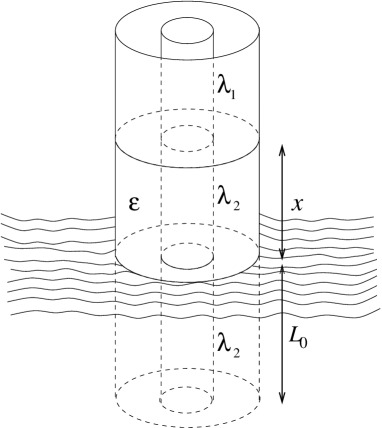
Figure 1: A cylindrical capacitor partially immersed in a tank containing a liquid dielectric. The liquid inside the capacitor rises when a potential difference is applied between the plates.

Let $L_{0}$ be the length of the capacitor that is immersed in the liquid before the voltage is turned on. After the voltage is turned on the liquid inside the capacitor rises to the height $L_{0}+x$ , as depicted in Fig 1. Let $\lambda_{1}$ and $\lambda_{2}$ be the linear charge densities on the parts of the inner plate that are in empty space and in contact with the dielectric, respectively. The corresponding electric fields in vacuum and inside the dielectric are

$${\bf E}_{1}=\frac{\lambda_{1}}{2\pi\epsilon_{0}s}\,{\hat{\bf s}}\,,\,\,\,{\bf E}_{2}=\frac{\lambda_{2}}{2\pi\epsilon s}\,{\hat{\bf s}}\,,$$ (1)

where ${\hat{\bf s}}$ is the radial unit vector and $\epsilon$ is the permittivity of the dielectric. The voltage $V$ applied to the capacitor is given by the radial line integral either of ${\bf E}_{1}$ or ${\bf E}_{2}$:

$$V=\int_{a}^{b}{\bf E}_{1}\cdot{\hat{\bf s}}\,ds=\frac{\lambda_{1}}{2\pi\epsilon_{0}}\ln\frac{b}{a}=\int_{a}^{b}{\bf E}_{2}\cdot{\hat{\bf s}}\,ds=\frac{\lambda_{2}}{2\pi\epsilon}\ln\frac{b}{a}\,.$$ (2)

From this the capacitance can be readily found. Indeed, the total charge of the capacitor is

$$Q=\lambda_{1}[L-(L_{0}+x)]+\lambda_{2}(L_{0}+x)=\frac{2\pi V}{\ln(b/a)}\bigl{\{}\epsilon_{0}[L-(L_{0}+x)]+\epsilon(L_{0}+x)\bigr{\}}\,,$$ (3)

whence

$$C=\frac{2\pi\epsilon_{0}}{\ln(b/a)}[L+\chi_{e}(L_{0}+x)]\,,$$ (4)

where $\chi_{e}$ is the electric susceptibility of the dielectric.

The force on the dielectric can be determined by equating the work done by the capacitor during a displacement $dx$ of the dielectric to the decrease of the electrostatic energy stored in the capacitor. Thus, assuming the charge $Q$ of the capacitor remains constant as the displacement takes place,

$$F=-\frac{dE}{dx}=-\frac{d}{dx}\bigg{(}\frac{Q^{2}}{2C}\bigg{)}=\frac{1}{2}\frac{Q^{2}}{C^{2}}\frac{dC}{dx}=\frac{\pi\epsilon_{0}\chi_{e}V^{2}}{\ln(b/a)}\,,$$ (5)

where Eq. (4) has been used. Since this force is positive, the dielectric is pulled into the capacitor. As is well known, the same result is obtained for the force if, instead of the charge $Q$, the voltage $V$ of the capacitor is assumed to remain constant during the displacement. But in the latter case the battery responsible for maintaining the voltage fixed does work as the dielectric is displaced, and this work must be taken into account in the energy balance [3]. Since the expression for the force is the same in both cases, it may seem obvious that the motion of the liquid dielectric does not depend on whether the charge or the voltage is held constant. This is not the case, however, for a reason that may be easily overlooked. If the voltage is held constant then the force (5) is constant during the entire motion. However, if the charge $Q$ remains constant then, using $V=Q/C$ and Eq. (4), the force (5) becomes

$$F=\frac{Q^{2}}{C^{2}}\frac{\pi\epsilon_{0}\chi_{e}}{\ln(b/a)}=\frac{Q^{2}}{4\pi\epsilon_{0}}\frac{\chi_{e}\ln(b/a)}{[L+\chi_{e}(L_{0}+x)]^{2}}\,.$$ (6)

This is a variable force that depends on the position of the dielectric because the capacitance increases and the voltage decreases as the dielectric penetrates the capacitor. Therefore, the dynamics of the dielectric is different depending on whether the charge or the voltage of the capacitor is constant throughout the motion.

III Equation of motion of the liquid dielectric

The equation of motion of the liquid dielectric is

$$\frac{d}{dt}(m{\dot{x}})=F+\rho gL_{0}\pi(b^{2}-a^{2})-mg$$ (7)

where $m$ is the mass of the dielectric that is already inside the capacitor at time $t$. The presence of the term proportional to $L_{0}$ on the right-hand side of (7) is justified as follows. The pressure at the bottom of the liquid column that is inside the capacitor is higher than the pressure at the top by $\rho gL_{0}$, where $\rho$ is the density of the dielectric. This gives rise to a net upward pressure force that equals $\rho gL_{0}\pi(b^{2}-a^{2})$ and must be added to the electrostatic force $F$. We have assumed that the area of the tank is much larger than $\pi(b^{2}-a^{2})$, so that the variation of the height of the liquid in the tank can be safely ignored. Other hypotheses will be mentioned in due time.

The mass of liquid inside the capacitor is

$$m=\pi(b^{2}-a^{2})(L_{0}+x)\rho\,.$$ (8)

Insertion of this expression for the mass into the equation of motion (7) leads to

$$\frac{d}{dt}\bigl{[}(L_{0}+x){\dot{x}}\bigr{]}=\frac{F}{\pi(b^{2}-a^{2})\rho}-gx\,.$$ (9)

IV Motion in the constant voltage case

If $V$ is constant, the use of (5) allows us to write Eq.(9) as

$$y{\ddot{y}}+{\dot{y}}^{2}+gy=gL_{0}+\frac{\epsilon_{0}\chi_{e}V^{2}}{\rho(b^{2}-a^{2})\ln(b/a)}\,.$$ (10)

where we have introduced the new variable $y$ defined by

$$y=L_{0}+x\,.$$ (11)

The task of solving equation (10) is made easier by writing it in dimensionless form. It is easy to check that the positive constants $a_{0}$ and $t_{0}$ defined by

$$a_{0}=\frac{\epsilon_{0}\chi_{e}V^{2}}{\rho g(b^{2}-a^{2})\ln(b/a)}=gt_{0}^{2}$$ (12)

have dimensions of length and time, respectively. In terms of the dimensionless variables $\xi$ and $\tau$, and dimensionless parameter $\alpha$, defined by

$$\xi=\frac{y}{a_{0}}=\frac{L_{0}+x}{a_{0}}\,,\,\,\,\tau=\frac{t}{t_{0}}\,,\,\,\,\alpha=\frac{L_{0}}{a_{0}}\,,$$ (13)

the differential equation (10) reduces to

$$\xi\frac{d^{2}\xi}{d\tau^{2}}+\bigg{(}\frac{d\xi}{d\tau}\bigg{)}^{2}+\xi=1+\alpha\,.$$ (14)

This equation has the equilibrium solution $\xi_{eq}=1+\alpha$, which is tantamount to $x_{eq}=a_{0}$. Thus, $a_{0}$ is the height at which the weight of the dielectric that has risen above the external level is exactly counterbalanced by the electric force that pulls it up.

Equation (14) can be solved by standard techniques. First of all we make a change of independent variable:

$$p=\frac{d\xi}{d\tau}\Longrightarrow\frac{d^{2}\xi}{d\tau^{2}}=\frac{dp}{d\tau}=\frac{dp}{d\xi}\frac{d\xi}{d\tau}=p\frac{dp}{d\xi}\,.$$ (15)

This reduces Eq.(14) to

$$\xi p\frac{dp}{d\xi}+p^{2}+\xi-1-\alpha=0\,,$$ (16)

or, in terms of differential forms,

$$\xi pdp+(p^{2}+\xi-1-\alpha)d\xi=0\,.$$ (17)

We seek an integrating factor $N(\xi)$ that turns the left-hand side of this equation into an exact differential:

$$N(\xi)\xi pdp+N(\xi)(p^{2}+\xi-1-\alpha)d\xi=dG\,.$$ (18)

Such a function $G(\xi,p)$ exists if and only if

$$\frac{\partial}{\partial\xi}[N(\xi)\xi p]=\frac{\partial}{\partial p}[N(\xi)(p^{2}+\xi-1-\alpha)]\Longrightarrow\xi\frac{dN}{d\xi}=N\,.$$ (19)

Thus, $N(\xi)=\xi$ is an integrating factor and we have

$$dG=\xi^{2}pdp+\xi(p^{2}+\xi-1-\alpha)d\xi\,.$$ (20)

The function $G$ can be readily found by integrating $dG$ along the broken path composed of the two straight line segments $(0,0)\to(\xi,0)\to(\xi,p)$, and one immediately gets

$$G(\xi,p)=\frac{1}{2}\xi^{2}p^{2}+\frac{\xi^{3}}{3}-\frac{1+\alpha}{2}\,\xi^{2}\,.$$ (21)

Therefore, the general solution of (16) is

$$\frac{1}{2}\xi^{2}p^{2}+\frac{\xi^{3}}{3}-\frac{1+\alpha}{2}\,\xi^{2}=C\,,$$ (22)

where $C$ is an integration constant.

IV.1 Close to the edge: a qualitative description

Equation (5) is adequate for the force only when the surface of the liquid is far from the edges of the capacitor. Therefore, it is not legitimate to put $L_{0}=0$ in equation (10). Nevertheless, something remarkable happens when one considers $L_{0}=0$. Since the attraction is caused by the fringing field, it is clear that the force on the liquid dielectric is not zero when its surface just touches the lower edge of the capacitor. Suppose that at $t=0$ the liquid is at rest, the voltage is turned on and the upward motion begins with $\xi=0$. Then the “first” ascending layer of the liquid has zero mass but is pulled into the capacitor with a finite force. Thus, ideally, it is subjected to an infinite acceleration, which brings about a finite jump of the velocity. Sure enough there is a transient process during which the electric field builds up and the velocity changes continuosly. However, since the time scale of this transient process is certainly much shorter than the time scale of the motion, it seems reasonable to expect that it can be satisfactorily modelled by a discontinuous jump of the velocity. Furthermore, the value attained by the velocity right after the transient, when so to speak the electrostatic force takes over, most likely cannot be freely chosen. This is a very peculiar behavior of this unconventional variable-mass system, whose mass can drop to zero at certain instants in the course of its motion.

It turns out that this unique behavior is nicely illustrated, at least in some of its main qualitative aspects, by our description. In order to check this statement let us try to find out what the equation of motion has to tell us about the dynamics of the liquid near the edge of the capacitor, although the quantitative results are admittedly unreliable.

With $\alpha=0$ because we are taking $L_{0}=0$, the initial condition $\xi(0)=0$ demands $p(0)=\pm 1$, as plainly seen from either (14) or (16). Accordingly, since $\xi$ starts to increase immediately after $t=0$, we take for initial conditions $\xi(0)=0$ and $p(0)=1$, a choice that leads to $C=0$ in equation (22). As a consequence, Eq.(22) can be solved for $p$ in the form

$$\frac{d\xi}{d\tau}=\sqrt{1-\frac{2}{3}\xi}\,\,\,\Longrightarrow\,\,\,\tau=\int_{0}^{\xi}\frac{d\lambda}{\sqrt{1-\frac{2}{3}\lambda}}=-3\sqrt{1-\frac{2}{3}\xi}+3\,.$$ (23)

This is easily inverted to yield

$$\xi(\tau)=\frac{9-(\tau-3)^{2}}{6}=\frac{\tau(6-\tau)}{6}\,.$$ (24)

It is clear that $\xi$ attains its maximum value $\xi_{max}=3/2$ at $\tau=3$, and returns to its initial value $\xi=0$ at $\tau=6$. Then $p$ changes abruptly from $p=-1$ to $p=1$ and the motion repeats itself, as shown in Fig. 2. The period of oscillation is $\tau_{0}=6$ in dimensionless units. These quantitative results are not trustworthy and the cusps at the turning points will be smoothed out in the actual motion, but the qualitative nature of the dynamics seems to be well represented by our description.

Figure 2: Periodic oscillation of the surface of the liquid dielectric near the bottom edge of the capacitor in terms of dimensionless quantities in the constant voltage case.

IV.2 Far from the edge: a quantitative description

Let us suppose now that $L_{0}\approx L/2$, where $L$ is the length of the capacitor, so that the liquid starts its motion well inside the capacitor. In this case our appoach is expected to be fairly realistic, and furnish quantitative results that can be taken seriously. If the fluid is at rest when the voltage is turned on, the initial conditions are $x(0)=0$ and ${\dot{x}}(0)=0$, which are equivalent to $\xi(0)=\alpha$ and ${\dot{\xi}}(0)=0$ according to equation (13). In this case the constant of integration is given by $\,C=\alpha^{3}/3-(1+\alpha)\alpha^{2}/2$ and equation (22) becomes

$$\frac{1}{2}\xi^{2}p^{2}+V(\xi)=0\,,\,\,\,\ V(\xi)=\frac{\xi^{3}-\alpha^{3}}{3}-\frac{1+\alpha}{2}\,(\xi^{2}-\alpha^{2})\,.$$ (25)

Recalling that $p=d\xi/d\tau$, this equation can be solved in the form

$$\tau=\frac{1}{\sqrt{2}}\int_{\alpha}^{\xi}\frac{z\,dz}{\sqrt{\frac{1+\alpha}{2}(z^{2}-\alpha^{2})-\frac{1}{3}(z^{3}-\alpha^{3})}}\,.$$ (26)

The appearence of the square root of a cubic polynomial in the above integrand indicates that the solution for $\xi(\tau)$ will be given by elliptic functions. However, much interesting information about the motion can be obtained without using these not so familiar functions. To this end note that equation (25) is formally equivalent to the one that describes the motion of a particle with zero “total energy” in the “potential” $V(\xi)$. The positivity of the “kinetic energy” $\xi^{2}{\dot{\xi}}^{2}/2$ constrains $\xi$ to the region $V(\xi)\leq 0$. Since $x\geq 0$, in terms of $\xi$ the physically allowed region is $\xi\geq\alpha$, as follows from Eq.(13).

The function $V(\xi)$ has the following properties: (i) $V(\alpha)=0$; (ii) $V^{\prime}(\alpha)=-\alpha<0$ which implies $V(\xi)<0$ for $\xi$ slightly bigger than $\alpha$; (iii) $V(\xi)\to\infty$ as $\xi\to\infty$; (iv) there is only one positive solution to $V^{\prime}(\xi)=0$, which is readily found to be $\xi_{eq}=1+\alpha$ and corresponds to $x_{eq}=a_{0}$. This result for $\xi_{eq}$ is merely a confirmation of what was found directly from the equation of motion (14). Now we have enough information to draw a qualitative graph of the “potential”, which is depicted in Fig. 3. The motion is confined to the “potential well” shown in the same figure.

Figure 3: Qualitative description of the periodic oscillation of the surface of the liquid dielectric in the constant voltage case. The dimensioless variable $\xi$ is confined in the “potential well” between $\xi=\alpha$ and $\xi=\xi_{max}$.

The amplitude of the oscillation of the surface of the liquid, that is, the maximum value attained by $\xi$ is the only positive value $\xi=\xi_{max}>\alpha$ such that $V(\xi)$ equals zero. In the region $\xi>\xi_{max}$ the “potential” is positive and the motion is forbidden. The amplitude $\xi_{max}$ is the positive solution to the algebraic equation

$$\frac{\xi^{3}-\alpha^{3}}{3}=\frac{1+\alpha}{2}(\xi^{2}-\alpha^{2})\,\,\Longrightarrow\,\,\frac{\xi^{2}+\alpha\xi+\alpha^{2}}{3}=\frac{1+\alpha}{2}(\xi+\alpha)\,,$$ (27)

since $\xi\neq\alpha$. This quadratic equation for $\xi$ is solved by

$$\xi_{max}=\frac{1}{4}\bigg{[}3+\alpha+3\alpha\,\sqrt{1+\frac{10}{3\alpha}+\frac{1}{\alpha^{2}}}\,\bigg{]}\,.$$ (28)

Typically, as will be seen presently, $L_{0}\gg a_{0}$, so that $\alpha\gg 1$. In this case a binomial expansion gives the following approximate expression for $\xi_{max}$:

$$\xi_{max}=\frac{1}{4}\bigg{[}\alpha+3+3\alpha\,\Bigl{(}1+\frac{5}{3\alpha}\Bigl{)}\,\bigg{]}=\alpha+2\,.$$ (29)

As a consequence, $x_{max}=2a_{0}$. Therefore the surface of the liquid dielectric inside the capacitor oscillates periodically between $x=0$ and $x=x_{max}=2a_{0}$. From (26) it follows at once that the period of oscillation is

$$T=\sqrt{2}\,t_{0}\,\int_{\alpha}^{\xi_{max}}\frac{\xi\,d\xi}{\sqrt{\frac{1+\alpha}{2}(\xi^{2}-\alpha^{2})-\frac{1}{3}(\xi^{3}-\alpha^{3})}}\,.$$ (30)

An expression for $T$ in terms of elliptic integrals is given in the Appendix.

Unfortunately, under normal laboratory conditions the oscillation of the surface of the liquid will be very hard to observe. In order to make $a_{0}$ and $t_{0}$ as large as possible, one needs a low-density liquid with very high susceptibility. Not only $a$ and $b$ but also their difference should be as small as possible, while the voltage should be as high as possible. However, these choices are limited, among other things, by the dielectric strength of the liquid. The dielectric strength of typical insulators [4] is about $10^{7}$ V/m. The maximum electric field inside the capacitor is easily seen to be $E_{max}=V/a\ln(b/a)$, so that one must have $V<10^{7}\,a\ln(b/a)$, with $a$ and $b$ in meters. Furthermore, the difference $b-a$ cannot be too small lest capillarity becomes dominant. To give an idea of the order of magnitudes involved, consider pure water, for which $\rho\approx 1\,\mbox{g/cm}^{3}$ and $\chi_{e}\approx 79$. Take $a=1.0\,\mbox{cm}$, $b=2.0\,\mbox{cm}$, $L=20\,\mbox{cm}$, $L_{0}=10\,\mbox{cm}$, and $V=5000$ volts, a very high voltage. Then from (12) and (13) we obtain $a_{0}=0.86\,$cm, $t_{0}=30\,\mbox{ms}$ and $\alpha=11.6$, so that $\xi_{max}=13.6$. It follows that the amplitude of the oscillation is $x_{max}\approx 2a_{0}=1.7\,\mbox{cm}$. The period of oscillation calculated in the Appendix is $T=0.93\,\mbox{s}$. It should be stressed that these values for the amplitude and the period require an extremely high voltage.

V Constant charge case

Making use of (6) the equation of motion (9) becomes

$$\frac{d}{dt}[(L_{0}+x){\dot{x}}]=\frac{\chi_{e}Q^{2}\ln(b/a)}{4\pi^{2}\epsilon_{0}\rho(b^{2}-a^{2})}\frac{1}{(L+\chi_{e}x)^{2}}-gx\,.$$ (31)

The same change of variables (13), but this time with $a_{0}$ and $t_{0}$ replaced by

$${\bar{a}}_{0}=\frac{\chi_{e}Q^{2}\ln(b/a)}{4\pi^{2}\epsilon_{0}\rho(b^{2}-a^{2})L^{2}g}\,\,\,,\,\,\,{\bar{t}}_{0}=\sqrt{\frac{\chi_{e}Q^{2}\ln(b/a)}{4\pi^{2}\epsilon_{0}\rho(b^{2}-a^{2})L^{2}g^{2}}}\,,$$ (32)

reduces equation (31) to the dimensionless form

$$\xi\frac{d^{2}\xi}{d{\tau}^{2}}+\left(\frac{d\xi}{d\tau}\right)^{2}+\xi=\alpha+\frac{1}{(1+\sigma\xi)^{2}},$$ (33)

where $\alpha=L_{0}/{\bar{a}}_{0}$ and the additional dimensionless parameter $\sigma$ is given by

$$\sigma=\frac{\chi_{e}{\bar{a}}_{0}}{L}\,.$$ (34)

The same procedure as in the previous case leads to the following first integral for Eq. (33):

$$\frac{\xi^{2}p^{2}}{2}+\frac{\xi^{3}}{3}-\frac{\alpha}{2}\xi^{2}-\frac{1}{\sigma^{2}}\left[\ln(1+\sigma\xi)+\frac{1}{1+\sigma\xi}\right]={\bar{C}}\,.$$ (35)

The initial conditions $\xi(0)=\alpha$, $p(0)=0$ determine ${\bar{C}}$. A qualitative description of the motion can be given following the pattern set by the previous case. The shape of the “potential” is exactly the same as the one shown in Fig. 3. The motion is periodic and confined to the interval $\alpha\leq\xi\leq{\bar{\xi}}_{max}$ where, now, ${\bar{\xi}}_{max}$ is determined by a transcendental equation because of the logarithmic term in (35), which prevents us from giving an explicit expression for the amplitude of the oscillation. The period is also given by a complicated integral involving the square root of a logarithm.

VI Conclusion

The motion of a liquid dielectric attracted by a vertical cylindrical capacitor is an unusual example of dynamics of a variable-mass system. As we have seen, because the initial mass vanishes for motion of the liquid near the lower edge of the capacitor with the most natural initial conditions, the velocity change can be qualitatively modelled by a jump determined by the equation of motion itself. Assuming that the surface of the liquid remains far from the ends of the capacitor, we exactly solved for the motion in the case of constant voltage and found not too complicated expressions for the amplitude and the period of the oscillation. If, instead, the charge of the capacitor is held constant, the motion is qualitatively the same but quantitative results are different, and demand more complicated numerical computations.

Appendix A The period in terms of elliptic integrals

According to (27) the “potential” $V(\xi)$ has the three real roots $\xi_{1}=\alpha$, $\xi_{2}=\xi_{max}\equiv\beta$, $\xi_{3}=-\gamma$, where

$$\beta=\frac{1}{4}\bigg{[}\alpha+3+3\alpha\sqrt{1+\frac{10}{3\alpha}+\frac{1}{\alpha^{2}}}\,\bigg{]}\approx\alpha+2\,,\,\,\gamma=\frac{1}{4}\bigg{[}3\alpha\sqrt{1+\frac{10}{3\alpha}+\frac{1}{\alpha^{2}}}-\alpha-3\bigg{]}\approx\frac{1+\alpha}{2}$$ (36)

and the approximate equalities hold if $\alpha\gg 1$. Thus we can write

$$-V(\xi)=\frac{1+\alpha}{2}\,(\xi^{2}-\alpha^{2})-\frac{\xi^{3}-\alpha^{3}}{3}=\frac{1}{3}(\xi-\alpha)(\beta-\xi)(\xi+\gamma)$$ (37)

and equation (30) for the period takes the form

$$T=\sqrt{2}\,t_{0}\int_{\alpha}^{\beta}\frac{x\,dx}{\sqrt{-V(x)}}=\sqrt{6}\,t_{0}\,\int_{\alpha}^{\beta}\frac{x\,dx}{\sqrt{(x-\alpha)(\beta-x)(\gamma+x)}}\equiv\sqrt{6}\,t_{0}\,I\,.$$ (38)

We follow [5] and perform the change of variable $x=\beta-u^{2}$, which leads to

$$I=2\int_{0}^{\sqrt{\beta-\alpha}}\frac{(\beta-u^{2})du}{\sqrt{(\beta-\alpha-u^{2})(\beta+\gamma-u^{2})}}\equiv 2\beta I_{1}-2I_{2}\,.$$ (39)

The additional change of variable $u=\sqrt{\beta-\alpha}\,\sin\theta$ reduces both integrals $I_{1}$ and $I_{2}$ to the standard form of complete elliptic integrals. Let us first tackle $I_{1}$:

$$I_{1}=\int_{0}^{\sqrt{\beta-\alpha}}\frac{du}{\sqrt{(\beta-\alpha-u^{2})(\beta+\gamma-u^{2})}}=\frac{1}{\sqrt{\beta+\gamma}}\int_{0}^{\pi/2}\frac{d\theta}{\sqrt{1-k^{2}\sin^{2}\theta}}\,,$$ (40)

that is,

$$I_{1}=\frac{1}{\sqrt{\beta+\gamma}}\,K(k)\,,\,\,\,k=\sqrt{\frac{\beta-\alpha}{\beta+\gamma}}$$ (41)

where $K(k)$ is the complete elliptic integral of the first kind. Similarly

$$I_{2}=\frac{\beta-\alpha}{\sqrt{\beta+\gamma}}\int_{0}^{\pi/2}\frac{\sin^{2}\theta\,d\theta}{\sqrt{1-k^{2}\sin^{2}\theta}}=\frac{\beta-\alpha}{\sqrt{\beta+\gamma}}\int_{0}^{\pi/2}\frac{-(1-k^{2}\sin^{2}\theta)/k^{2}+1/k^{2}}{\sqrt{1-k^{2}\sin^{2}\theta}}d\theta\,,$$ (42)

so that

$$I_{2}=\frac{\beta-\alpha}{k^{2}\sqrt{\beta+\gamma}}\bigg{[}\int_{0}^{\pi/2}\frac{d\theta}{\sqrt{1-k^{2}\sin^{2}\theta}}-\int_{0}^{\pi/2}\sqrt{1-k^{2}\sin^{2}\theta}\,d\theta\bigg{]}=\sqrt{\beta+\gamma}\,\Bigl{[}K(k)-E(k)\Bigr{]}\,,$$ (43)

where $E(k)$ is the complete elliptic integral of the second kind.

After some simplifications, we finally get

$$T=2\sqrt{6}\,t_{0}\,\bigg{\{}\sqrt{\beta+\gamma}\,E(k)-\frac{\gamma}{\beta+\gamma}K(k)\bigg{\}}\,.$$ (44)

The functions $K(k)$ and $E(k)$ are given by the following power series ($0\leq|k|<1$):

$$K(k)=\int_{0}^{\pi/2}\frac{d\theta}{\sqrt{1-k^{2}\sin^{2}\theta}}=\frac{\pi}{2}\bigg{\{}1+\bigg{(}\frac{1}{2}\bigg{)}^{2}k^{2}+\bigg{(}\frac{1\cdot 3}{2\cdot 4}\bigg{)}^{2}k^{4}+\bigg{(}\frac{1\cdot 3\cdot 5}{2\cdot 4\cdot 6}\bigg{)}^{2}k^{6}+\ldots\bigg{\}}\,;$$ (45)

$$E(k)=\int_{0}^{\pi/2}\sqrt{1-k^{2}\sin^{2}\theta}\,d\theta=\frac{\pi}{2}\bigg{\{}1-\bigg{(}\frac{1}{2}\bigg{)}^{2}k^{2}-\bigg{(}\frac{1\cdot 3}{2\cdot 4}\bigg{)}^{2}\,\frac{k^{4}}{3}-\bigg{(}\frac{1\cdot 3\cdot 5}{2\cdot 4\cdot 6}\bigg{)}^{2}\,\frac{k^{6}}{5}+\ldots\bigg{\}}\,.$$ (46)

For the parameters chosen in the main text we have seen that $\alpha=11.6$. Then (36) yields $\beta=13.6$ and $\gamma=6.26$. With these values the modulus of the complete elliptic integrals is found from (41) to be $k=0.317$. For this $k$ the values for the complete elliptic integrals furnished by the above power series are $K(k)=1.6125$ and $E(k)=1.5306$. Finally, with $t_{0}=30\,\mbox{ms}$ equation (44) gives $T=0.93\,\mbox{s}$.

References

• [1] J. A. Stratton, Electromagnetic Theory (McGraw-Hill, New York, 1941), pp. 137-153; L. Landau et E. Lifchitz, Γ‰lectrodynamique des Milieux Continus (Mir, Moscou, 1969), sections 15 and 16.
• [2] E. R. Dietz, Force on a dielectric slab: Fringing field approach, Am. J. Phys. 72, 1499-1500 (2004).
• [3] D. J. Griffiths, Introduction to Electrodynamics (Prentice Hall, New Jersey, 1999), 3rd edition, section 4.4.4.
• [4] W. E. Forsythe, Smithsonian Physical Tables (Lord Baltimore Press, Baltimore, 1959), Table 434, p. 423.
• [5] M. R. Spiegel, Advanced Calculus (McGraw-Hill, New York, 1963), chapter 16.