Unstable Optical Resonators & Fractal Light


MSci Project Report
Jarvist Moore Frost
(email: jarvist.frost@ic.ac.uk)

Abstract

Codes were written to simulate the propagation of monochromatic light through a bare optical resonator, using a computational Fourier method to solve the Huygens-Fresnel integral. This was used, in the Fox-Li method, to find the lowest-loss eigenmodes of arbitrary cavity designs. An implicit shift ‘hopping’ method was employed to allow a series of increasingly higher-loss eigenmodes to be found, limited in number by computational time.

Codes were confirmed in their accuracy against the literature, and were used to investigate a number of different cavity configurations.

In addition to confirming the fractal nature of eigenmodes imaged at the conjugate plane of a symmetric ($g<-1$) resonator, an initial study was made of how the (imperfect) quality of the fractal fit varied as the defining aperture was moved around the cavity.

A comparison was also made with the fractal-patterns produced by codes written to simulate basic video-feedback.

1 Theoretical Groundwork

1.1 Optical Resonators

The simplest optical resonator consists of two curved mirrors set up facing each other. We can define some useful quantities known as g-factors that define the behaviour of the beam in terms of spacing and radius of curvature of the mirrors [Eqn. 1]. These are a scale independent way of defining the behaviour of the cavity.

$$g_{1}\equiv 1-\frac{L}{R_{1}}\qquad g_{2}\equiv 1-\frac{L}{R_{2}}$$ (1)

1.2 Stability Condition

A stable cavity is one in which (by a simple geometric argument) any light ray in the cavity will be trapped between the mirrors and redirected towards the centre of the cavity.

This condition can be easily defined in terms of the g-factors [Eqn. 2] and gives rise to a region on a $g_{1}vs.g_{2}$ plot that corresponds to stable cavity configurations.

$$0\leq g_{1}g_{2}\leq 1$$ (2)

When the g-factors exceed this region, a round-trip of the cavity becomes overall magnifying, and light inevitably ‘spills’ over the edge of the mirrors.

1.3 Transverse Eigenmodes

By considering a short pulse or ‘slab’ of radiation indefinitely recirculating between the mirrors of the cavity, and demanding that the transverse beam pattern be unchanged by propagation (i.e. a stable ‘lasing’ beam) one can identify a transverse pattern of the field that supports such indefinite oscillations without changing. This is known as the Transverse Eigenmode.

The action of the optical resonator can be considered as a matrix operator $\uuline{M}$ which modifies the transverse profile of the wavefront $U$. This leads to a basic eigenvalue equation:

$\uuline{M}U_{n}=\gamma_{n}U_{n}$

Finding the eigenmodes of an optical resonator is simply a matter of solving this equation. However, $\uuline{M}$ is not a simple linear operator but corresponds to the physical evolution of light (including diffraction effects) as it passes around the cavity.

These $U_{n}$ show a certain transverse (across the cavity) distribution that is very strongly dependent on varying cavity design. There are many such eigenmodes for a given cavity. The higher the order mode, the greater the round-trip loss of energy.

1.4 Geometrically Stable Cavities & Hermite-Gaussian Modes

In stable optical resonators, the eigenmodes produced are essential plane waves, multiplied by a transverse mode function. When expanded in rectangular transverse coordinates, these modes are given almost exactly by Hermite-Gaussian functions[9].These are often referred to as $TEM_{n,m}$ waves[9].

The transverse distribution of light intensity resembles a combination of Gaussian distributions. Therefore the majority of energy in the beam is concentrated in only a small region of the gain medium, leaving most of the gain underutilised.

1.5 Planar Resonators

The planar resonator occupies the [1,1] point of the g-factor stability diagram, and as such it might be considered somewhat surprising that stable eigenmodes exist on this boundary. The analytic treatment is far more difficult than for stable cavities, but in appearance the Eigenmodes are very similar to the $TEM$ modes, with the addition of Bessel functions adding diffraction ripples.

Unlike in a confocal resonator, these modes do not go to zero at the mirror edges, and a quantity of light is lost around the edges.

1.6 Unstable Cavities

Due to the positive magnification on each round trip of the cavity, a large proportion of the energy is lost past the mirror - in fact this can form a useful ‘doughnut’ output beam. Analytic expressions for the mode patterns are difficult to find, and it is these cavity designs which we used for the majority of our project.

Unstable Cavities have a number of benefits for high-power laser systems, including far better utilisation of the bulk of the gain-medium.

1.7 Virtual Source Technique

By unfolding the mirrored cavity into a series of effective apertures and lenses, the modal pattern can be inferred from taking a weighted sum of the edge diffraction effects & the non-diffracted plane wave passing through[10].

However, this technique has been mainly developed for square or $1D$ slit apertures[4], and so with the far more complicated mirror shapes that we hope to study, we will be forced to take an entirely numerical approach.

1.8 Huygens’ Integral

By considering the propagation of a light beam as the combination & interference of spherical Huygens’ wavelets originating at the source, the light field at any observable location can be derive. By considering a paraxial beam, where the distance between input & output planes is considered large enough so that $cos\theta\approx 1$ and utilising a simplified Paraxial-Spherical form of propagating wavelets, one can form the Fresnel approximation to Huygens’ integral[9].

This is made further useful for us by separating it into two one-dimension integrals [Eqn. 3][9].

$$\tilde{u}(x,y)=\sqrt{\frac{j}{L\lambda}}\int{\tilde{u}_{0}(x_{0}\,z_{0})exp(-j\frac{\pi(x-x_{0})^{2}}{L\lambda})dx_{0}}$$ (3)

This form of the integral represents a convolution of the input field $\tilde{u}_{0}$ with a spherical wave-function $exp(-j\pi x_{0}^{2}/(z-z_{0})\lambda)$. Convolution can be easily achieved by Fourier-transforming the two functions, doing a product multiplication of the results, then inverse Fourier transforming to produce the desired convolution[9].

This process can then be repeated for a given laser cavity with suitable interacting gain medium, until convergence on a ‘steady state’ modal pattern is observed[11] which can be considered an eigenmode of the given cavity.

1.9 Ray Matrices

Within the paraxial treatment, the effect of a number of optical elements (such as thin lenses, mirrors etc.) can be considered as items that modify the slope & displacement of incoming light beams by linear transformation. Therefore, one can define a rank 2 tensor (ray matrix) that acts upon a ray vector to transform it into what is present after the optical element.

When multiple elements are cascaded together, an overall ray matrix can be calculated by simply taking the normal matrix product of the constituent elements, algebraically arranging the ray matrices in inverse order to that which the ray physically encounters the elements[9].

Huygens’ Integral can be generalised to an equation that includes the Ray Matrix of an overall system (even allowing for complex ray matrix coefficients)[9], and which describes the entire paraxial propagation of light through the system, including any diffraction (but not aperture) effects. Limiting apertures (such as those forming the polygonal mirrors of our cavity) require propagation of light to this plane, then spatial filtering to produce the apertures.

1.10 Polygonal Mirrors & Nonorthogonal Basis

Previous studies have used a nonorthogonal basis[4] to describe the field intensity across the cavity. This allows polygonal and rhombus aperture shapes to be described exactly by the discretised mesh, whereas a standard Cartesian discretisation would necessitate a far finer mesh to describe the aperture with sufficient accuracy, and to not introduce significant errors from the ‘jagged edges’.

This introduces complications in the numerical code, as Huygens’ integral takes on a modified Fourier form, such as the ‘Hankel’ transform encountered when using cylindrical coordinates[9]. As this causes considerable constraints in choice of aperture shapes, and is fundamentally more difficult to visualise what is occurring, we decided to stick with a Cartesian grid.

2 Relevant Previous Studies

Previous work[4], utilising a Fourier convolution method to solve the Huygens’ integral, have been used to investigate unstable cavities with small Fresnel number $N_{eq}$ and linear magnifications of $1\leq M\leq 2$, with detailed study of the 8 lowest loss eigenmodes of $M=1.3$ cavities.

In order to produce eigenmodes of fractal nature, target mirrors of regular polyhedral & rhomboid shape were constructed. The produced mode patterns show self-similar structure, with higher $N_{eq}$ factors leading to a more complex & developed fractal structure. The fractal dimension of these patterns were found to be $1\leq D\leq 2$, embedded in the $2D$ transverse plane of the cavity.

2.1 Experimental Work

A prototype laser, utilising modified Iris diagrams to produce an aperture of variable size & shape, has been constructed from a He-Xe laser[2]. Evidence was found of the excess noise factor $K$ depending highly on aperture shape and $N_{eq}$, as would be expected when producing fractal mode patterns, but there is little direct experimental evidence of fractal structure in a laser beam.

3 Numerical Methods

Though the equations and methods used in our numerical simulation are present in the standard text[9], there were many subtleties and nuances encountered when implementing a working system. Most infuriatingly, there are many different ways of formulating the equations into a form suitable for solution on a computer - and it was difficult to separate descriptions of the general method from specifics of one implementation! This section along with consultation of the codes in Appendix A should allow one to quickly built a working code base.

3.1 Fox-Li Power Method

The Power method[9] is a very simple concept from linear algebra. When given any eigensystem, the repeated action of the operator (physical propagation around a cavity) on an initial eigenvector (the field distribution) will eventually lead to convergence if the system has a dominant eigenvalue[8]. The mode found will be the one with the highest absolute eigenvalue, corresponding to the lowest-loss case. Convergence can be extremely slow, in particular when one is in a region where two eigenvalues are nearly the same strength - a ‘mode crossing’. Also, repeated action of the operator will cause the eigenvector (field profile) to tend asymptotically to either $\inf$ or $0$. Scaling of the light intensity after every round-trip is necessary to keep the values at some sensible (and therefore more accurate) level.

As such, to find the lowest-loss mode pattern one simply needs to devise a system for propagating light around a cavity and then apply repeatably until converging at an eigenmode.

3.2 Light Propagation

The Huygens-Fresnel integral [Eqn. 3] can be described as a convolution operation. Propagating light from one reference frame to the next is achieved by summing contributions to the electric field from all the Huygens wavelets. With a discretised grid of $n$ units, this requires computational time of $O\approx n^{2}$ in $1D$, $O\approx n^{4}$ in $2D$ and quickly becomes intractable.

Convolution in real-space becomes a product in the Fourier domain, which brings enormous computational savings. A more innate physical understanding is garnered by interpreting the Fourier transform of a field profile as a collection of infinitely wide plane waves with varying angle to the normal of the reference plane (Fig. 1). These can then be propagated (in either direction) by making an allowance for the different path-lengths travelled by the waves. This involves applying a phase change equivalent to the extra distance that non-axial rays have to travel to reach the new plane. The light field distribution can then be recovered by undertaking an inverse Fourier transform.

Figure 1: Propagation of off axis rays introduces a phase retardation proportional to the extra distance that the ray has to travel

The path difference (Fig. 1) is first approximated in the paraxial approximation to be equal to the difference parallel to the plane of the optical cavity and then the circular arc of equi-distance is approximated as a parabola. Therefore, the extra length of a non-axis plane wave is proportional to $L\lambda k^{2}$, with $k$ being the spectral angle.

$$\zeta_{0}(k_{i},k_{j}) = \mathbb{F}(\eta_{0}(i,j))$$ (4)

$$\zeta_{1}(k_{i},k_{j}) = \zeta_{0}(k_{i},k_{j})e^{i\pi L\lambda(k_{i}^{2}+k_{j}^{2})}$$ (5)

$$\eta_{1}(i,j) = \mathbb{F}^{-1}(\zeta_{1}(k_{i},k_{j})$$ (6)

3.2.1 Implementation

We used the high-performance FFTW[6] library routines to undertake our Fast Fourier Transforms (FFTs). In spite of the high efficiency, the FFT step was found to be by far the most time-consuming step of running the simulation, which meant that none of our code was particularly speed critical.

Our FFT routines were found to require a rescaling to conserver energy of $\eta_{1}=\frac{\eta_{0}}{N}$ in $1D$ and $\eta_{1}=\frac{\eta_{0}}{N^{2}}$ in $2D$ after every application of a pair of transform & inverse transform. Like many Fast-Fourier-Transform methods FFTW[6] flips the placement of high & low spectral frequencies for performance reasons. Rather than waste time remapping these into a scratch buffer, modulo arithmetic was used to rearrange the array lookups in situ whilst working in the Fourier domain.

When working on a $NxN$ discretised grid with a full-width aperture size $A$ and $\frac{N}{2}$ locating the axis of propagation, we need to do the following in the Fourier domain:

$out[i][j]*=cexp(i\pi\frac{L*\lambda}{A^{2}}(((i+\frac{N}{2})\%N-\frac{N}{2})^{2}+((j+\frac{N}{2})\%N-\frac{N}{2})^{2});$

3.2.2 FFT Guard Bands

The FFT is not a true Fourier transform (which is an integral from $-\infty$ to $+\infty$), but an infinite series of finite integrals. Within the framework of considering the physical interpretation of the mathematics, this can be visualised as an infinite series of screens onto which the light is imaged. As can be seen (fig. 2) one needs to use use a Guard Band around the edges of the usefully-propagated region, in order to stop spillover from adjoining cells.

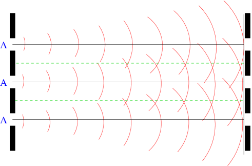
Figure 2: The finite nature of the Discrete Fourier Transform results in an infinite series of propagating waveforms, either side of the (dotted) region one is using. As such, light can leak across from either side, producing an incorrect field distribution.

The requirement of this $G$ factor can be indicated [11] by considering the amount of light spilling from a single aperture uniformly illuminated due to a combination of the overall geometric magnification and an edge diffraction pattern.

This spillover is proportional to the equivalent Fresnel number $N_{eq}$ and the magnification of the setup. With esoteric cavity designs we found that the actual required $G$ factor generally far exceeded this amount (and was even influenced by the shape of the aperture in $2D$). In general we confirmed the sufficiency of the guard bands by varying them slightly and seeing if there was any change of the supposed eigenmode produced.

The maximum energy spillover was found to be less than $10^{-2}$ for reliable eigenmode formation.

The most elegant and simple test of the propagation subroutine was to generate a test Gaussian wavefront, then propagate varying distances to confirm that the standard beam propagation relations were reproduced.

3.3 Lensing

Our optical cavity is unfolded into an infinite series of thin lenses & free-space propagation. In the paraxial approximation, with a mirror surface that causes no overall phase-shift to the reflected light and with perfectly aligned optics, a lens is simulated by that of a phase shift proportional to the square of the distance from the optical axis, scaled to produce correct focal-point effect (fig. 3).

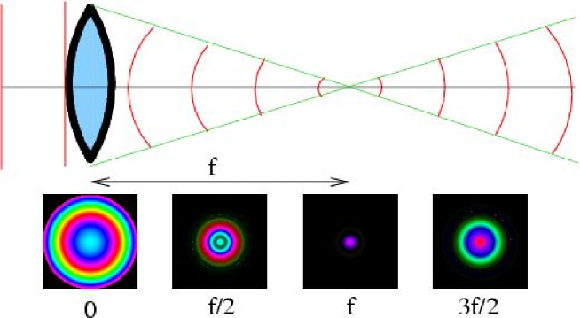
Figure 3: Effect of an infinitely thin lens is to induce a spherical curvature to the wavefront, resulting in a hitherto parallel collection of rays converging on it. The $2D$ pictures below (colour representing phase, intensity representing intensity) are data from our codes, which show a circular cross-section plane wave focusing down to a diffraction limited spot near the focal point, before expanding again.

Mathematically, what we are doing in the Spatial domain is:

$u_{1}(i,j)=u_{0}(i,j)e^{\frac{i\pi}{f\lambda}(i^{2}+j^{2})}$

On a discretised grid of $NxN$ units, with a full-width aperture of $A$, this corresponds to pseudo-code of:

$ap[i][j]*=cexp(\frac{i\pi}{f\Lambda}\frac{A^{2}}{N^{2}}((i-\frac{N}{2})^{2}+(j-\frac{N}{2})^{2}));$

3.3.1 Testing Correctness

The main mechanism to test the effect of lensing was to apply a lens to plane-parallel light, then propagate forwards to various points (most importantly, the focal length $f$ and the image point $2f$) to confirm that the correct behaviour was observed. In $2D$ with a ‘square’ chunk of light, the focusing effect was lost amid pronounced edge diffraction, whereas a circular beam of plane light was far more elegant (fig. 3).

3.4 Bare Optical Resonator

A basic bare optical resonator is one in which two mirrors face each other across a non-interacting medium. In terms of our simulation, we unfold these two mirrors into an infinite series of thin lenses & propagation over free-space (fig. 4).

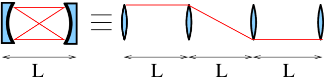
Figure 4: Unfolded optical cavity.

For a situation where the defining aperture is one of the mirrors (such as most unstable cavities) it is possible to condense any combination of intervening optical elements into a single ABCD matrix. This can then be expanded into an ‘equivalent lens guide’[9] of lens & free-space (Fig. 4). This results in a vast saving in computational time, as each ABCD element with a non zero B component (representing some free-space propagation) otherwise requires two FFTs. For a two-mirror cavity setup with one mirror defining the aperture of the system this doubles the speed of calculation.

Though there are methods[9] of incorporating a general ABCD matrix directly into the Huygens-Fresnel integral, we found it better to use an equivalent Lens & Free-Space infinite series, as we found it far easier to debug and visualise what was going on. We soon garnered an intuitive grasp of how requirements of minimum discretisation ($N$) and guard bands ($G$) varied with different cavities.

3.5 Detection of Eigenmodes

The Fox-Li method will eventually deliver the simulation at an eigenmode, whereupon Eqn. 7 is held. It is essential to be able to detect when an eigenmode has been reached, and derive a quantitative figure for the eigennumber of the mode ($\gamma$).

$$\uuline{M}\eta_{n}=\gamma_{n}\eta_{n}$$ (7)

The spatial variation of the field remains unchanged after a round-trip of the cavity - however, it is necessary for there to be an overall phase change & energy loss associated with the eigenmode. This can be represented as the $\gamma$ factor, a complex scalar by which all the points making up the spatial representation of the eigenmode are multiplied by to arrive at the exact pattern produced after one more round-trip.

The unchanging nature of the gamma factor upon successive round trips, and the fact that all points across the spatial domain have to simultaneously obey it when at an eigenmode was used to simultaneously detect eigenmodes and quantify $\gamma$. After each round trip of the cavity, the average $\gamma$ factor was calculated by comparing each $\eta_{1}(i,j)$ with $\eta_{0}(i,j)$, ignoring positions corresponding to relatively small values of $\eta$ with the justification that the error in $\gamma$ would scale with $\frac{1}{\eta}$. Once this average $\gamma$ figure was calculated, it was compared with all the individual $\gamma(i,j)$ measurements. An eigenmode was detected if none of the $\gamma(i,j)$ figures disagreed with the overall $\gamma$ factor by more than a certain tolerance, generally taken to be $1$ part in $10000$.

This method was found to be very flexible and established the most accurate possible $\gamma$ factor. The tolerance was derived experimentally, set at a point where the ‘eigenmodes’ produced no longer varied with a changing tolerance value. It was generally found that convergence on the first eigenmode came within $100$ passes for an unstable cavity configuration, but exceptional cases near mode-crossings could take up to $1000$ passes.

3.5.1 Implicit Shift

The basic Fox-Li power method is only capable of finding the lowest loss eigenmode for the resonator. In order to allow higher-loss modes to be found, one must somehow cancel the presence of the dominant lower modes.

This can be accomplished by using knowledge of the $\gamma$ factor associated with a given mode to destroy the contribution of that mode in the overall pattern. Considering the measured light field as a summation of various eigenmodes, then after one round trip we will a field of these modes multiplied by their respective $\gamma$ factors:

$$\eta_{0} = u_{1}+u_{2}+u_{3}+u_{4}\ldots$$ (8)

$$\eta_{1} = \gamma_{1}u_{1}+\gamma_{2}u_{2}+\gamma_{3}u_{3}+\gamma_{4}u_{4}\ldots$$ (9)

If we take our round-trip profile $\eta_{1}$ and subtract a known $\gamma_{1}\eta_{0}$ factor (using the previously found $\gamma$ and the prior light field distribution), then we will destroy any presence of the this eigenmode in $\eta_{1}$. However, since this step can never be perfect (due to inaccuracy in our estimation of $\gamma$) and the natural tendency of the system to want to generate the lowest-loss eigenmode - we must apply this cancellation repeatably during the simulation. Each mode that we find gives us another $\gamma$ factor that we can apply in succession in order to find higher modes. This is equivalent to the Shift method in linear algebra[8].

The most effective method of mode-searching that we found was to iterate in successive round-trips of the cavity over a ‘carousal’ of the found $\gamma$ factors, then allow a number of normal unperturbed round trips (generally $10$) to see if a new eigenmode would stabilise before already-known lower-loss eigenmodes arose from the background noise. For instance, if we consider there to be an error of $\sigma$ associated with each $\gamma$ factor, and a carousal of three known eigenmodes the process will be:

$$\eta_{0} = u_{1}+u_{2}+u_{3}+u_{4}\ldots$$ (10)

$$\eta_{1} = \sigma_{1}u_{1}+\gamma_{2}u_{2}+\gamma_{3}u_{3}+\gamma_{4}u_{4}\ldots$$ (11)

$$\eta_{2} = \sigma_{1}\gamma_{1}^{2}u_{1}+\sigma_{2}u_{2}+\gamma_{3}^{2}u_{3}+\gamma_{4}^{2}u_{4}\ldots$$ (12)

$$\eta_{3} = \sigma_{1}\gamma_{1}^{3}u_{1}+\sigma_{2}\gamma_{2}u_{2}+\sigma_{3}u_{3}+\gamma_{4}^{3}u_{4}\ldots$$ (13)

$$\eta_{4} = \sigma_{1}\gamma_{1}^{4}u_{1}+\sigma_{2}\gamma_{2}^{2}u_{2}+\sigma_{3}\gamma_{3}u_{3}+\gamma_{4}^{4}u_{4}\ldots$$ (14)

Clearly - new modes stop being found once the error in $\sigma$ is such that the higher-loss higher-order mode is never able to dominate (i.e. when $\sigma_{1}\gamma_{1}^{n-1}\approx\gamma_{i}^{n}$). Modes often require a number of such cycles to become dominate & be identified but even imperfect mode cancellation allows the $u_{n}$ part of the overall $\eta$ distribution to be sufficiently strong so that it stabilises to an eigenmode.

3.6 Polygon Apertures

A method was sought to be able to easily produce regular polygon apertures. The best method found was to use a standard point inclusion in polygon test [5], then fill in an aperture mask using this selection criteria.

3.7 Outputs

A simple data format was used containing tab-separated values for the various measurements across the middle of the aperture (or along the infinitely thin slice when running in $1D$). These values included the location $x$, complex and imaginary parts of $\eta$, the intensity ($I\alpha\eta^{2}$) and phase ($\phi_{x}=atan\frac{\Im(\eta_{x})}{\Re(\eta_{x})}$).

The $\eta$ field variation across the centre of a $2D$ square aperture should agree exactly with a $1D$ infinitely thin slit with identical cavity configuration. This was used as an indicator that the overall $2D$ functioning was correct.

3.7.1 Representing Phase & Intensity

In order to show both phase and intensity information in one figure, a routine was written to output colour representations of the transverse light field, with the ‘brightness’ of the pixel representing the intensity, and the phase ($0\to 2\pi$) sampling a colour from a standard $HSV$ colour wheel[12], with no phase ($\phi=0$) as cyan. These could then easily be separated at a later date into monochrome intensity plots (desaturation) or pure phase plots (full saturation).

3.8 Sampling Fractal Dimension

There are a number of, seemingly contradictory, methods of defining the fractal dimension of a particular object ($D$). As we are dealing with graphs (the transverse eigenmodes) with an unclear relationship between the scaling of the physical dimension versus the intensity, simple box counting methods are less than ideal. A method of calculating the Hurst exponent using the rescaled range was found to be the easiest to implement and was implemented in our codes.

The Hurst exponent can be considered a measurement of the persistence of the function - the extent to which it is predictable. Fractal dimension, for a $2D$ graph is related by:

$$D=2-H$$ (15)

A predictable linear varying function will have a Hurst exponent of 1 (range scales directly with sample size) and therefore a fractal dimension of 1 - it is a $1D$ object embedded in a $2D$ graph. Conversely, the more complexity in the mode pattern, the lower the Hurst exponent and the higher fractal dimension. However - pure noise has a Hurst coefficient of zero, implying the highest possibly degree of fractal structure. Therefore, though Hurst analysis can be used to quantify the degree of fractal structure, it is not sufficient to declare whether a particular structure is a (self-similar) fractal or not.

4 Results

4.1 Equivalent Confocal Cavity

A general cavity can be converted into an equivalent confocal form by placing the $ABCD$ matrix between two opposite lenses. This can then be easily unfolded into an equivalent lens guide, allowing one to halve the computational effort necessary to locate eigenmodes. We generally investigated symmetric cavities ($g_{1}=g_{2}$).

Eigenvalues are located on a convex hull in the complex plain, but due to the way that the carousal-algorithm ‘hops’ shifts the origin on the plane, the modes are not discovered in strict order of lowest loss but that each found eigenmode is the one furthest away (therefore greatest in magnitude) from the $\gamma$ values being used to suppress the lower order eigenmodes.

A typical set of eigenvalues is represented (fig. 5), along with the associated $2D$ plots (fig. 6). Weak self similar structures are demonstrated in these transverse patterns, with the structure of the aperture (an n-side polygon) being replicated at smaller and smaller scales.

Figure 5: Gamma factors for the first 15 Eigenmodes of a low-magnification symmetric cavity ($M=1.1$) with a hexagonal limiting aperture. Each ‘spoke’ of the wheel represents the gamma factor of the eigenmode, the square of the length of which (the absolute value of the complex $\gamma$ factor) represents the energy retained after each round trip in this eigenmode.

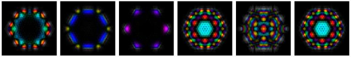
Figure 6: Intensity plots of the 6 lowest loss eigenmodes from (fig. 5); colour is phase of light on HSV[12] colour wheel.

4.2 Confirmation of Codes Accuracy

In order to assure that our codes were finding eigenmodes correctly, we replicated data from the literature, in particular Fig. 4 of [7]). This consisted of locating lowest-loss eigenmodes for a symmetric cavity with magnifications $1.8$ & $1.9$, using a relatively low equivalent Fresnel number of $49.4$. Agreement is extremely good, and gave us confidence in the ability of our codes to find accurate eigenmodes.

Figure 7: Intensity mode-profiles for a $1D$ (and similarly, cross section on square aperture $2D$) unstable confocal cavity with $M=2.8$,$2.9$. $N_{eq}=49.4$

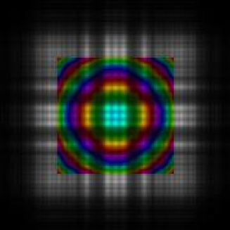
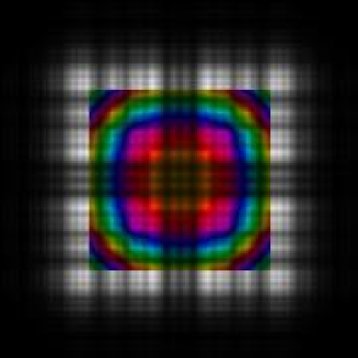
Figure 8: Corresponding transverse $2D$ plots.

4.3 The Conjugate Plane

Considering a symmetric cavity, with $g<-1$, one can identify by a simple ray tracing argument the existence of two conjugate planes. These planes $U^{\prime}$ & $V^{\prime}$ image onto each other after a half-trip of the cavity (with a magnification of the half-trace of the cavity: $m=\sqrt{M}$), and onto themselves after a full round trip of the cavity (Fig. 9).

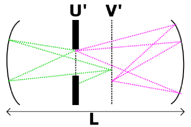
Figure 9: Location of the $U^{\prime}$ and $V^{\prime}$ conjugate planes in a confocal cavity, by a simple ray tracing argument.

With the simple case of where the defining aperture of the cavity is at one of the mirrors, and then propagating to a suitable conjugate plane, one discovers that the pattern of the eigenmodes bare a very clear fractal character. In fact, if one overlaps the mode pattern against a Magnification-factor stretched version of itself (Fig. 10), there is extremely good agreement in pattern (peaks and troughs) but not the magnitude of the eigenmode.

Perhaps this should not be too surprising - by its very definition, the $U^{\prime}$ and $V$ planes are self-imaging, but do so with a round trip magnification. Any eigenmode rendered at the image plane will have to obey such a situation, and so must display a self-similar nature.

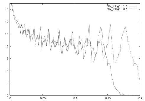
Figure 10: Eigenmode projected to $U^{\prime}$ conjugate plane, plotted against a $M$ stretched version of itself - showing clear self similarity. $N_{eq}=49.4$, $M=1.3$.

Generating these modes was extremely computationally demanding, the cavity setup requiring an extremely large FFT Guard Band, far in excess of what is predicted by considering the $N_{eq}$ & $M$ parameters. This is believed to be due to the naive (non ABCD equivalent lens guide) stepwise method by which we propagated light around these more complex cavities.

As such this was even slower in $2D$ but we did manage to capture a lowest-loss eigenmode11. Curiously, there was no pattern observable in the phase information whatsoever - just uniform circular fringes. The reasons for this are not well understood.

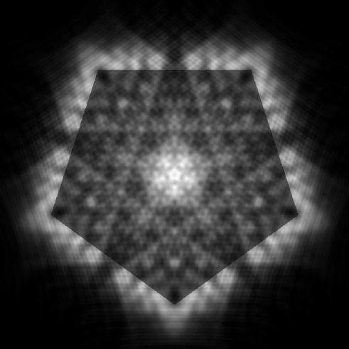
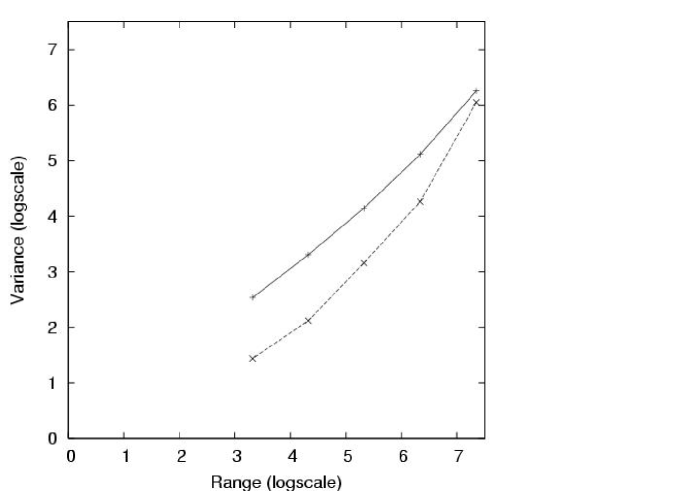
Figure 11: $2D$ Intensity plot and Hurst analysis of first eigenmode at conjugate plane with $M=1.3$, $N_{eq}=49.4$. The Pentagonal aperture has been slightly toned to allow its location; that pattern does not really exist in the eigenmode.

The Hurst analysis for a $1D$ eigenmode (Fig. 11) with identical cavity parameters, at both the aperture defining mirror (shallow line) and conjugate plane (steeper line) shows a clear difference between Hurst coefficients. The eigenmode rendered at the conjugate plane has a fractal dimension of $D=1.977$, whereas at the aperture mirror $D=1.84$. The conjugate plane possesses a far higher degree of fractal structure, which confirms the qualitative appreciation of the ‘stretched fit’ (Fig. 10).

4.4 Moving the Location of the Aperture

The fractal eigenmode produced at the conjugate plane is not perfect. It was hypothesised that this was due to the defining aperture of the system occurring at a non-self-imaging location, and that the quality of the fractal would be increased by moving the limiting aperture to the imaging plane.

However, this was found to be a numerically impossible situation to simulated - as the $ABCD$ matrix evaluated for the round trip between the image plane and itself has a zero B value. This corresponds to there being no effective distance between the two planes, and an infinite equivalent Fresnel number.

In order to avoid this numerical impossibility, we attempted to shift the aperture towards the complex pattern, and see whether an improvement in the fractal fit of the eigenmode occurred. We produced some qualitative evidence for this increase in fractal quality as the aperture shifted towards the conjugate planes, but were limited from quantifying it by an inability to define mathematically how good the fractal fit actually was, especially as $N_{eq}\to+\infty$ and so the amount of patterning increased.

5 Video Feedback

A number of articles[1][3] draw a parallel between the fractals character of unstable resonator modes, and the patterns produced by a ‘Monitor-Outside-a-Monitor’ pixelated video feedback. The process of geometric magnification in the two systems is the same, but instead of having the Huygens-Fresnel (Eqn. 3) to select which part of the field contributes to the next intensity distribution (i.e. the vector sum of the Cornu spiral), a pixel-function is defined that allows for the overlap & finite size of pixels.

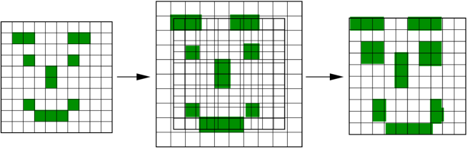
Figure 12: Schematic of Video-Feedback.

As shown in Fig. 12, the ‘pixel-function’ defines the way in which the magnified pixels of one frame influence the pixels produced in the next frame. Each successive frame is comprised of a magnification of the previous pattern, with distorted edge effects (caused by the mismatched grid overlap) that have a clear parallel with edge diffraction ripples occurring in a cavity simulation.

With a simple ‘perfect’ grid pixel function, no fractal behaviour is demonstrated. Real video fractals occur due to the pixel structure (the finite size of the photo-sensitive element in the CCD grid) causing an uneven overlay of the grid. The perfect grid situation is equivalent to the geometric limit of the cavity simulation - where no diffraction effects take place and no patterned eigenmode exists.

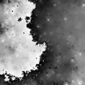
Figure 13: Typical video-feedback ‘eigenmode’ - imprecise fractal self-similarity expressed on the ‘curved coastline’. $M=1.4$, $p_{width}=0.65$ & $M=1.3$, $p_{width}=0.6$ respectively.

There wasn’t enough time for the codes written simulating video-feedback to acquire sufficient finesse (in particular with the definition of the pixel function) to be able to make direct quantitative predictions of real cavity eigenmodes such as has been demonstrated in [1] However very similar behaviour was observed in both simulated video feedback & the laser cavity simulation. In particular, first order eigenmodes (Fig. 13) with fractal character are readily established by running light around the feedback system (i.e. in a parallel to the Fox-Li power method), which are entirely indifferent to starting conditions, suggesting that they result from the underlying setup of the feedback system rather than the initial field distribution.

6 Conclusions

A set of flexible and efficient codes were produced that could accurate predict eigenmodes produced in an arbitrary & easily-specified bare optical resonator configuration using the Fox-Li power method. Higher order modes could be located (at computational expense) by the shift-method. The codes can seamlessly change between $1D$ and $2D$ cavities with $n-sided$ regular polygon mirrors.

The vast majority of time in the project was taken up in developing these codes and proving them qualitatively against the literature, leaving little time to actually use them to explore the behaviour of unstable resonator modes.

However, we clearly demonstrated that some unstable modes have self-similar characteristics, that an n-sided polygon aperture has that motif repeated at smaller and smaller sizes in the eigenmode and that a far higher quality of fractal eigenmode is rendered by projecting to an image plane in a symmetric $g<-1$ resonator.

Further work could use these codes to study the conjugate plane in greater detail, and attempt to derive would would occur in a real system with the aperture creating an infinite equivalent Fresnel number situation. The biggest stumbling block that we found to this was to find a suitably rigorous way of defining how accurate the M-stretched pattern (Fig. 10) matched itself. We investigated using a least-squares method to compare, but due to the lack of magnitude conservation in the stretched pattern, we found it would be necessary to use some kind of rescaled range at the very least. Alternatively, one could break down the pattern into a simplified description - such as locating the peaks & troughs, then comparing these; or using a spectral (FFT) method to investigate self-similarity in the bandwidth occupied by the pattern. There is also the unresolved issue of considering how to counteract the effect of the increasing Fresnel number in the calculations.

These codes could also be used to investigate what happens at the stability boundaries on the g-factor diagram, investigating whether the transition from stable to unstable modes is as truly sharp as suggested in the reference texts[9].

Codes were developed to simulate a basic Video-Feedback system, and the fractal nature & ability of a system to develop eigenmodes independent of the starting field distributions was demonstrated. Further work could develop these into a (far faster) method of predicting eigenmodes for an optical cavity[1], and could even be used to ‘seed’ a standard Fox-Li power method near an eigenmode such as is commonly done to improve accuracy of Prony & VS eigenmodes.

Appendix A Cavity Simulator Codes

⬇

/* Cavity Sim

* MSci Physics Project QOLS07, Imperial College

* Jarvist Frost & Benjamin Hall 2005-2006

*/

#include <complex.h>

#include <fftw3.h>

#include <math.h>

#include <stdio.h>

#include <stdlib.h>

#include <time.h>

#include ”pnpoly.c” //points in a polygon detection code

//#define TWO_DIMENSIONAL

#define N (1024*16)

#define G (0.2) //guard band - expressed as fraction of grid we SHOULD uss

#define TOLERANCE 0.0001 //tolerance of points in testing for eigenmode

#define SAMPLEPOINTS 200 //number of random points to sample to test for Eigenmode

#define MAX_EIGENS 10

#define SPACERS 10 //number of non-shift applying ’spacers’ in eigenvalue meth

#define A 1.414E-2 //was 1mm

double L = 1.0; //3.14; //was 0.001

double FOCAL = -100000;

double LAMBDA= 10e-08; //1.0E-7; //0.4488E-6; //0.11225E-6; //0.069754E-6; //0.067349E-6; //0.069754E-6 //1 micron

int CROP=1; //crop output photos?

fftw_plan fft, fftr;

double M;

#define R 500000.0 //radius curvature gaussian spherical beam

#define WAIST 1E-3 //waist of g.s. beam

#ifdef TWO_DIMENSIONAL

fftw_complex ap[N][N];

fftw_complex out[N][N];

fftw_complex old_ap[N][N];

int filter[N][N];

#endif

#ifndef TWO_DIMENSIONAL

fftw_complex ap[N][1];

fftw_complex out[N][1];

fftw_complex old_ap[N][1];

int filter[N][1];

#endif

double RS[N];

fftw_complex gamma_shift[MAX_EIGENS];

fftw_complex gamma_old, gamma_new;

struct coord

{

int x, y;

} samples[SAMPLEPOINTS];

double rescaled_range(int start, int length);

double hurst();

void input_ap_picture (void);

void output_ap_slice (char *name);

void output_ap_picture (char *name);

void aperture_filter (void);

void propogate (double LENGTH);

void normalise_intensity_in_cavity (void);

void generate_initial_intensity ();

void scale_fft(); //correct for scale caused by FFT routines

void

input_ap_picture ()

{

char buffer[200];

int i, j, p;

FILE *fo;

fo = fopen (”in.raw”, ”r”);

/* fscanf(fo,”%s\n”,&buffer);

fscanf(fo,”%s\n”,&buffer);

fscanf(fo,”%s\n”,&buffer);

fscanf(fo,”%s\n”,&buffer);

*/

for (i = 0; i < N; i++)

for (j = 0; j < N; j++)

{

fscanf (fo, ”%d\n”, &p); //red

// fscanf(fo,”%d\n”,&p); //green

// fscanf(fo,”%d\n”,&p); //blue

ap[i][j] = (double) p;

// printf(”%d %d %d\n”,i,j,p);

}

fclose (fo);

}

void

output_ap_slice (char *name)

{

int i,j=0;

FILE *fo;

#ifdef TWO_DIMENSIONAL

j=N/2; //take slice across centre if in 2D, otherwise just read out 1D array

#endif

fo = fopen (name, ”w”);

fprintf (fo, ”#index creal cimag cabs cabs*cabs\n”);

for (i = N/2; i < N; i++)

fprintf (fo, ”%f %f %f %f %f %f %f\n”, (double)(i-N/2)/((double)N*G*0.5/sqrt(2)),

(double)(i-N/2)/((double)N*G*0.5/sqrt(2))*sqrt(M),

(double)(i-N/2)/((double)N*G*0.5/sqrt(2))*M,

creal (ap[i][j]),

cimag (ap[i][j]), cabs (ap[i][j]),

cabs(ap[i][j]*ap[i][j]) );

fclose(fo);

}

void

output_ap_picture (char *name)

{

double scr = 0.0, sci = 0.0, phi, s, v, p, q, t, f, r, g, b;

int i, j, mag, magmax = 0, Hi;

int size,bottom,top;

FILE *fo;

fo = fopen (name, ”w”);

// fprintf(stderr,”Output Apperture to: %s\n”,name);

if (CROP==1)

{

// size=(int)((float)N*G);

size=N/2;

bottom=N/4;

top=3*N/4;

// bottom=1+(int)((1-G)*(float)N/2);

// top=N-(int)((1-G)*(float)N/2);

}

else

{

size=N; bottom=0; top=N;

}

fprintf (fo, ”P6\n%d %d\n%d\n”, size, size, 254);

for (i = 0; i < N; i++) //calculate scale factor

for (j = 0; j < N; j++)

{

if (cabs (ap[i][j]) * cabs (ap[i][j]) > scr)

scr = cabs (ap[i][j]) * cabs (ap[i][j]);

/* if (cimag(ap[i][j])>sci)

sci=cimag(ap[i][j]);*/

}

for (i = bottom; i < top; i++)

//apply scale factor to normalise amount of light in cavi$

{

for (j = bottom; j < top; j++)

{

phi = M_PI + atan2 (cimag (ap[i][j]), creal (ap[i][j]));

// phi=2*M_PI*(cabs(ap[i][j])*cabs(ap[i][j]))/scr;

s = 1.0;

v = (cabs (ap[i][j]) * cabs (ap[i][j])) / scr;

// v=1.0;

// printf(”HSV: %f %f %f\n”,phi,s,v);

//HSV->RGB formula from http://en.wikipedia.org/wiki/HSV_color_space

Hi = (int) (floor (phi / (M_PI / 3.0))) % 6;

f = phi / (M_PI / 3.0) - floor (phi / (M_PI / 3.0));

p = v * (1.0 - s);

q = v * (1.0 - f * s);

t = v * (1.0 - (1.0 - f) * s);

if (Hi == 0)

{

r = v;

g = t;

b = p;

}

if (Hi == 1)

{

r = q;

g = v;

b = p;

}

if (Hi == 2)

{

r = p;

g = v;

b = t;

}

if (Hi == 3)

{

r = p;

g = q;

b = v;

}

if (Hi == 4)

{

r = t;

g = p;

b = v;

}

if (Hi == 5)

{

r = v;

g = p;

b = q;

}

// printf(”%f\n”,f);

if (filter[i][j] != 0) //if we’re displaing the mask…

r = g = b = v; //make it greyscale!

fprintf (fo, ”%c%c%c”, (int) (254.0 * r), (int) (254.0 * g),

(int) (254.0 * b));

// fprintf(fo,”%d %d %d ”,65535-mag,65535-mag,65535-mag);

}

}

fclose (fo);

}

void

make_filter (int nsides)

{

int i, j, n;

float x[100], y[100];

double grad, xinit;

//first draw a circle

/* for (i=0;i<N;i++) for (j=0;j<N;j++)

if ((float)((i-N/2)*(i-N/2)+(j-N/2)*(j-N/2)) > (G*G*(float)N/2.0*(float)N/2.0))

filter[i][j]=1; //masked

else

filter[i][j]=0; //not masked*/

//then draw polygon within circle by chopping off edges

#ifdef TWO_DIMENSIONAL

for (n = 0; n < nsides; n++)

{

x[n] =

N / 2 -

G * (N / 2) * cos ((M_PI/(double)nsides)+ (double) n * (2.0 * M_PI / (double) nsides));

y[n] =

N / 2 +

G * (N / 2) * sin ((M_PI/(double)nsides)+(double) n * (2.0 * M_PI / (double) nsides));

}

for (i = 0; i < N; i++)

for (j = 0; j < N; j++)

if (pnpoly (nsides, &x[0], &y[0], (float) i, (float) j))

filter[i][j] = 0;

else

filter[i][j] = 1;

#endif

#ifndef TWO_DIMENSIONAL

for (i = 0; i < N; i++)

{

if (i<N/2-(G*(N/2)/sqrt(2)) || i>N/2+(G*(N/2)/sqrt(2)))

filter[i][0]=1;

else

filter[i][0]=0;

}

#endif

}

void

aperture_filter ()

{

int i, j=0;

for (i = 0; i < N; i++)

#ifdef TWO_DIMENSIONAL

for (j = 0; j < N; j++)

#endif

if (filter[i][j] != 0) //do this with unary logic

ap[i][j] = 0.0 + 0.0I;

}

void

propogate (double LENGTH)

{

int i, j=N/2; //set j at centre of cavity

double shift;

fftw_execute (fft);

for (i = 0; i < N; i++) //plane wave propogation

#ifdef TWO_DIMENSIONAL

for (j = 0; j < N; j++)

//we need to use the modulus operator to flip the quadrants -

// the FFT algo changes location of the high-spectral freq

out[i][j] *= cexp ( I * M_PI*

(1.0/(double)A)*(1.0/(double)A)*

(double)

(((i + N / 2) % N - N / 2) *

((i + N / 2) % N - N / 2) +

((j + N / 2) % N - N / 2) *

((j + N / 2) % N - N / 2))

* ( LENGTH * (double)LAMBDA));

#endif

#ifndef TWO_DIMENSIONAL

out[i][0] *= cexp ( I * M_PI*

(1.0/(double)A)*(1.0/(double)A)*

(double)

(((i + N / 2) % N - N / 2) *

((i + N / 2) % N - N / 2))

* ( LENGTH * (double)LAMBDA));

#endif

/* for (i=0;i<N;i++) //Apply Hanning Window to spectral form

for (j=0;j<N;j++

out[i][j]*= 0.54-0.46 *

cos(2*M_PI*i/(N-1))*cos(2*M_PI*j/(N-1));

*/

fftw_execute (fftr);

scale_fft(); //corrects for scale in FFT algorithm

}

void lens(double f) //apply spherical lens curvature to wavefrount

//i.e. phase retardation dependent on distance from axis

{

int i,j=0;

for (i = 0; i < N; i++)

#ifdef TWO_DIMENSIONAL

for (j = 0; j < N; j++)

ap[i][j] *=

cexp (I

*M_PI

/ ((double)f*(double)LAMBDA)

* (((double)A/(double)N) * ((double)A/(double)N)) *

(double) ((i - N / 2) * (i - N / 2) +

(j - N / 2) * (j - N / 2)));

#endif

#ifndef TWO_DIMENSIONAL

ap[i][0] *=

cexp (I

*M_PI

/ ((double)f*(double)LAMBDA)

* (((double)A/(double)N) * ((double)A/(double)N)) *

(double) ((i - N / 2) * (i - N / 2) ));

#endif

}

void

normalise_intensity_in_cavity ()

{

double sc = 0.0;

int i, j=0;

for (i = 0; i < N; i++) //calculate scale factor

#ifdef TWO_DIMENSIONAL

for (j = 0; j < N; j++)

#endif

if (filter[i][j]==0) //if within aperture

sc += cabs (ap[i][j])*cabs(ap[i][j]);

sc=(double)sc; //discard imaginery part

#ifdef TWO_DIMENSIONAL

sc=sc/((double)N*(double)N*G*G); //average abs. value of pixel in cavity

#endif

#ifndef TWO_DIMENSIONAL

sc=sc/((double)N*G);

#endif

sc=sqrt(sc); //take sqrt to get

// fprintf(stderr,”Normalise intensity: sc %f\n”,sc);

for (i = 0; i < N; i++) //apply scale factor to normalise amount of light in cavity

#ifdef TWO_DIMENSIONAL

for (j = 0; j < N; j++)

#endif

ap[i][j]=ap[i][j]/sc;

}

void

generate_initial_intensity ()

{

int i, j=0;

for (i = 0; i < N; i++)

#ifdef TWO_DIMENSIONAL

for (j = 0; j < N; j++)

#endif

{

// ap[i][j]=(i-N/2)+((j-N/2)*I);

/* if (i>0.25*N

&& i<0.75*N

&& j>0.25*N

&& j<0.75*N )

ap[i][j]=1.0+0.0I;

else

ap[i][j]=0.0+0.0I;

*/

ap[i][j] = cexp (

// -I*2*M_PI/LAMBDA*

// ((double)((i-N/2)*(i-N/2)+(j-N/2)*(j-N/2))/(double)(N))

// /R

-

(A*A)* ((double)

((i - N / 2) * (i - N / 2) +

(j - N / 2) * (j - N / 2))

/ (double) (N * N)) /

(WAIST*WAIST));

ap[i][j] = 1.0 + 0.0I; //DIRTY! :)

// fprintf(stderr,”i: %d j: %d\t%f + %f i\n”,i,j,creal(ap[i][j]),cimag(ap[i][j]));

}

}

void scale_fft() //correct for scale caused by FFT routines

{

int i,j;

for (i = 0; i < N; i++)

#ifdef TWO_DIMENSIONAL

for (j = 0; j < N; j++)

ap[i][j]/=(double)N*(double)N; //correct for scaling of FFT algo

#endif

#ifndef TWO_DIMENSIONAL

ap[i][0]/=(double)N; //correct for scaling of 1D FFT algo

#endif

}

void

output_filter ()

{

int i, j;

for (i = 0; i < N; i++)

for (j = 0; j < N; j++)

ap[i][j] = 1.0;

aperture_filter ();

}

fftw_complex calculate_gamma()

//Calculate Gamma shift factor by comparing average of succesive pixels once stabilised on eigenmode

{

int i,j=0,ap_points = 0;

fftw_complex gamma_new=0.0;

for (i = 0; i < N; i++)

#ifdef TWO_DIMENSIONAL

for (j = 0; j < N; j++)

#endif

if (filter[i][j] ==0 && cabs(ap[i][j])>0.05)

{

ap_points++;

gamma_new += ap[i][j] / old_ap[i][j];

}

gamma_new /= (double) ap_points;

// fprintf(stderr,”%d”,ap_points);

return(gamma_new);

}

void apply_gamma_shift(int shift)

{

int i,j=0;

for (i = 0; i < N; i++)

#ifdef TWO_DIMENSIONAL

for (j = 0; j < N; j++)

#endif

ap[i][j] -= old_ap[i][j] * gamma_shift[shift]; //rotate between gamma_shift shifts on each successive pass

//So - just what are we meant to do here? Apply subtractive shift to previous frame?

// fprintf(stderr,”Apply Gam: %f + %f I\n”,creal(gamma_shift[1+passes%eigenmode_count])

// ,cimag(gamma_shift[1+passes%eigenmode_count]));

}

double hurst(char *name)

//Derived from equations at

// http://www.bearcave.com/misl/misl_tech/wavelets/hurst/index.html

{

FILE *fo;

int i=0,n;

int bits=0,size=512;

double data[20][2];

double avg;

double extent=0.4; //fraction of guard band we’ll be using

size=(int)(extent*G*N)/2.0;

printf(”%d\n”,size);

fo = fopen (name, ”w”);

bits=size;

while (bits>=8)

{

avg=0.0;

for (n=0;n<size;n+=bits)

avg+=rescaled_range(n+N/2,bits);

avg/=(double)(size/bits); //was size/bits

fprintf(fo,”%f %f %f %f\n”,1.0/(double)bits,avg,log((double)bits)/log(10.0),log(avg)/log(10.0));

data[i][0]=log((double)bits)/log(10.0); data[i][1]=log(avg)/log(10.0);

i++;

bits/=2;

}

fprintf(fo,”#D: Approx: %f\n”,(data[0][1]-data[i-1][1])/(data[0][0]-data[i-1][0]) );

fclose(fo);

return(0.0); //FIXME

}

double rescaled_range(int start, int length)

//Dervied from equations at

// http://www.bearcave.com/misl/misl_tech/wavelets/hurst/index.html

{

int i;

double avg=0.0,min=0.0,max=0.0,sd=0.0;

for (i=start;i<start+length;i++)

avg+=(double)cabs(ap[i][0]);

avg/=(double)length; //calculate avg. value

RS[0]=0.0;

for (i=1;i<=length;i++)

{

RS[i]=RS[i-1]+(double)cabs(ap[i+start][0])-avg;

if (RS[i]<min) min=RS[i];

if (RS[i]>max) max=RS[i];

}

for (i=start;i<start+length;i++)

sd+=((double)cabs(ap[i][0])-avg)*((double)cabs(ap[i][0])-avg);

sd/=(double)length; //now contains variance

sd=sqrt(sd); //now S.D.

return ((max-min)/sd);

}

main ()

{

int i, j=0, k, l, passes, n, eigenmode_flag, eigenmode_count, ap_points,shift;

int framecount=0;

char name[100],tmp[100];

double tmpr, tmpi, sc, total_error,Neq,conjugate_plane;

double gimag,greal;

double g1,g2,FOCAL_CONVERSION; //g-factors for laser cavity

#ifdef TWO_DIMENSIONAL

fft = fftw_plan_dft_2d (N, N,

&ap[0][0], &out[0][0], FFTW_FORWARD, FFTW_ESTIMATE);

fftr = fftw_plan_dft_2d (N, N,

&out[0][0],

&ap[0][0], FFTW_BACKWARD, FFTW_ESTIMATE);

#endif

#ifndef TWO_DIMENSIONAL

fft = fftw_plan_dft_2d (N, 1,

&ap[0][0], &out[0][0], FFTW_FORWARD, FFTW_ESTIMATE);

fftr = fftw_plan_dft_2d (N, 1,

&out[0][0],

&ap[0][0], FFTW_BACKWARD, FFTW_ESTIMATE);

#endif

srand (time (NULL));

fprintf (stderr, ”Plans created…N:%d\n”,N);

// for (M=1.5;M<1.6;M+=0.6)

for (n = 5; n < 6; n++) //n-sided polygon for aperture

// for (FOCAL = -2.0; FOCAL > -20.0; FOCAL -= 1.0)

{

// g1= -1.0526; //-1.01; //-1.055;

g1=-1.01;

// g1=-1.002;

// M=1.9;

// g1=(M+1.0) /(2.0*M);

g2=g1;

printf(”g1=%f g2=%f\n”,g1,g2);

// FOCAL=(-M*L)/((M-1)*(M-1));

// FOCAL=0.225;

FOCAL_CONVERSION=-g2*L/(g2-1);

FOCAL=1/(2-2*g1);

conjugate_plane=(L/2)*sqrt((g1+1)/(g1-1)); //distance x from centre of cavity

M=(-g1+sqrt(g1*g1 - 1))/(-g1-sqrt(g1*g1-1)); //Magnification of cavity

Neq=12.0;

LAMBDA=((M*M)-1)/(2*M)*(A*G*A*G/8.0)/(L*Neq); //choose lambda from previous Neq

fprintf(stderr,”Lamda: %e Neq: %f\n”,LAMBDA,Neq);

Neq=((M*M)-1)/(2*M) * (A*G*A*G/8.0)/(L*LAMBDA); //calculate Neq from A,Lambda,L & M

fprintf(stderr,”Congjugate planes: u:%f v:%f M: %f x: %f\n”,L/2-conjugate_plane,L/2+conjugate_plane,M,conjugate_plane);

//EQUIVALENT LENSGUIDE CONVERSIONS

// FOCAL=-(g2*L)/(2*(g1*g2-1)); //focal length of equiv lensguide - Eqn 16, GHCN notes

// L=2*g1*L; //equivalennt freescale length - Eqn 15, GHCN notes

fprintf(stderr,”M: %f L: %f Focal: %f Focal_Conversion %f N: %f Neq: %f\n”,

M,L,FOCAL,FOCAL_CONVERSION,

(0.5*A*G*0.5*A*G/2.0)/(L*LAMBDA),

//((1-L/FOCAL)-1)/2.0 *(0.5*A*G*0.5*A*G/2.0)/(L*LAMBDA));

Neq);

// ((M-1)/2.0 * (A*G*A*G/8.0)/(L*LAMBDA)));

// for (i=0;i<N;i++) for (j=0;j<N;j++)

// shift[i][j]=0.0+0.0I;

make_filter (n);

fprintf (stderr, ”Npolygon: %d M: %f Focal: %f\n”, n, M,FOCAL);

// for (L=0.001;L<=0.024;L+=0.001) //10 240 10

// {

// fprintf(stderr,”Going for Length %f\n”,L);

// input_ap_picture(); //Lena

//

gamma_old = gamma_new = 0.0 + 0.0I;

for (i = 0; i < N; i++)

#ifdef TWO_DIMENSIONAL

for (j = 0; j < N; j++)

#endif

old_ap[i][j] = 0.0 + 0.0I;

// for (greal=-1.0;greal<1.0;greal+=0.1)

// for (gimag=-1.0;gimag<1.0;gimag+=0.1)

// {

eigenmode_count = 0;

// gamma_shift[0]=greal+gimag*I;

generate_initial_intensity ();

// sprintf(name,”%.10d.pnm”,0);

// output_ap_picture(name);

// sprintf(name,”%.10d.log”,0);

// output_ap_slice(name);

aperture_filter ();

// lens(-FOCAL_CONVERSION);

for (passes = 0; passes < 10000; passes++)

{

// fprintf(stderr,”Nsides: %d Passes %d\n”,n,passes);

// sprintf(name,”%.10d.pnm”,framecount++);

// output_ap_picture(name);

//EQUIV LENSGUIDE

// lens(FOCAL);

// propogate (L);

lens(FOCAL);

propogate(L/2-conjugate_plane);

aperture_filter();

propogate(L/2+conjugate_plane);

lens(FOCAL);

propogate(L/2+conjugate_plane);

aperture_filter();

propogate(L/2-conjugate_plane);

//propogate(L);

//Gamma shift application

//Start of SHIFT selection

/* the following code applies the shifts in a straight series

* with a gap of SPACERS between each rotated application.

* So it looks like abc……abc…..abc…. etc.

*/

shift=(passes+(SPACERS-1))%(SPACERS+eigenmode_count) - SPACERS;

// if (shift>=0)

// shift=eigenmode_count-shift-1;

// fprintf(stderr,” %d ”,shift);

/* the following code applies the shifts in rotation, spaced by

* a gap of SPACERS between each single application of a shift.

* So it looks like a……b……c……a……b……c…. etc.

*/

/* if (passes%SPACERS==0 && eigenmode_count>0)

shift=(passes/SPACERS)%eigenmode_count;

else

shift=-1;

*/

//End of SHIFT selection

if (shift<0) { fprintf(stderr,”.”); sprintf(tmp,”X”);}

else

{

fprintf(stderr,”%c”,’a’+shift);

for (i=1;i<=shift+1;i++)

tmp[i]=’A’+i-1;

tmp[shift+2]=0;

apply_gamma_shift(shift);

}

gamma_new = calculate_gamma();

framecount++;

// sprintf(name,”%.10d_%s_Mode:%d_G:%f+%fI.pnm”,framecount,tmp,eigenmode_count,creal(gamma_new),cimag(gamma_new));

// output_ap_picture(name);

// normalise_intensity_in_cavity ();

// sprintf(name,”%.5d.pnm”,framecount);

// output_ap_picture(name);

// output_ap_slice(name);

// exit(-1);

/* printf(”G_new %f + %fI cabs: %f old:new %f\n”,

creal(gamma_new),cimag(gamma_new),

cabs(gamma_new),

cabs(gamma_new-gamma_old)

);

*/

if ( passes>15 && cabs (gamma_new - gamma_old) < (double) TOLERANCE) //see if stabailised to eigenmode by non-varying Gamma shift

{

fprintf (stderr, ”c@%d\n”, passes);

// fprintf(stderr,”Convergence to Eigenmode, with %f Tolerance.\n”,TOLERANCE);

gamma_shift[eigenmode_count] = gamma_new; //save gamma into shift table

printf (”Avg Gamma[%d]: %f + %fI\tAbs:%f\n”, eigenmode_count,

creal (gamma_shift[eigenmode_count]),

cimag (gamma_shift[eigenmode_count]),

cabs(gamma_shift[eigenmode_count]));

sprintf(name,”%dr.log”,eigenmode_count);

output_ap_slice(name);

sprintf(name,”h%d.log”,eigenmode_count);

hurst(name);

//remove the following cludge

/* lens(FOCAL);

propogate (L);

lens(FOCAL_CONVERSION);

propogate (-(0.5-conjugate_plane));

*/

// lens(FOCAL_CONVERSION); //back to full cavity

lens(1/(2-2*g1)); //FOCUS as actually mirror

propogate(0.5+conjugate_plane); //propogate forwards

normalise_intensity_in_cavity ();

sprintf(name,”%du_lr.log”,eigenmode_count);

output_ap_slice(name);

sprintf(name,”hc%d.log”,eigenmode_count);

hurst(name);

#ifdef TWO_DIMENSIONAL //if making a 2D eigenmode, output the pretty eigenmode!

sprintf(name,”%du_lr.pnm”,eigenmode_count);

output_ap_picture (name);

#endif

aperture_filter();

propogate (2*conjugate_plane);

sprintf(name,”%dv_lr.log”,eigenmode_count);

output_ap_slice(name);

propogate(0.5-conjugate_plane);

lens(1/(2-2*g1)); //FOCUS as actually mirror

propogate(0.5-conjugate_plane);

sprintf(name,”%dv_rl.log”,eigenmode_count);

output_ap_slice(name);

propogate (2*conjugate_plane);

sprintf(name,”%du_rl.log”,eigenmode_count);

output_ap_slice(name);

#ifdef TWO_DIMENSIONAL //if making a 2D eigenmode, output the pretty eigenmode!

sprintf(name,”%du_rl.pnm”,eigenmode_count);

output_ap_picture (name);

#endif

eigenmode_count++; //keep count of already discovered eigenmodes

passes = 0; //reset passes so we have full range to settle to next mode

gamma_old=gamma_new=0.0+0.0I; //reset gamma factors

}

aperture_filter ();

normalise_intensity_in_cavity ();

for (i = 0; i < N; i++)

#ifdef TWO_DIMENSIONAL

for (j = 0; j < N; j++)

#endif

old_ap[i][j] = ap[i][j];

// memcpy(old_ap,ap,sizeof(fftw_complex)*N*N);

gamma_old = gamma_new;

if (eigenmode_count >= MAX_EIGENS) //once we’ve gathered this many modes

break; //break out the for-loop!

}

fprintf (stderr, ”Reset\n”);

// }

// sprintf(name,”npoly%d_Foc%f_passes%.5d.pnm”,n,FOCAL,passes);

// output_ap_picture(name);

// output_ap_slice((int)(L*1000));

}

fftw_destroy_plan (fft);

fftw_destroy_plan (fftr);

}

Appendix B Video Fractal Codes

⬇

/* Jarvist Frost 2004-2006

* Program to create ’video-fractals’

*/

//#include <file.h>

#include <stdio.h>

#include <math.h>

#include <limits.h>

#define MAG (1.4)

#define X_RES 500

#define Y_RES 500

#define X_OFF 0 //offset of newcenter in pixels

#define Y_OFF 0

#define TWIST 3.14/6 //radians twist between zoom’s

#define PIXW 0.65 //0.65 //width of sensor pixel in display pixels

#define BACKGROUND 140

int curpic[X_RES][Y_RES];

int newpic[X_RES][Y_RES];

void outputpic(char *filename);

void inputpic(char *filename);

main()

{

int x,y,loops;

char filename[20];

//fill display with white noise

srand(123);

for (x=0;x<X_RES;x++)

for (y=0;y<Y_RES;y++)

curpic[x][y]=rand();

inputpic(”begin.pgm”);

outputpic(”first.pgm”);

// zoom();

// swap();

// outputpic(”test2.pgm”);

for(loops=0;loops<150;loops++)

{

printf(”%d\n”,loops);

sprintf(filename,”pic%.3d.pgm”,loops);

if (loops%10==0)

outputpic(filename);

zoom(); swap();

}

outputpic(”last.pgm”);

}

swap()

{

int x,y,max=0;

double light;

for (x=0;x<X_RES;x++)

for(y=0;y<Y_RES;y++)

{

curpic[x][y]=newpic[x][y];

if (curpic[x][y]>max)

max=curpic[x][y];

}

for (x=0;x<X_RES;x++)

for(y=0;y<Y_RES;y++)

curpic[x][y]*=INT_MAX/max;

}

zoom()

{

int x,y;

double nx,ny,np,dx,dy,r,theta,phi;

for (x=0;x<X_RES;x++)

for(y=0;y<Y_RES;y++)

{

dx=(0.5+(double)(x-(X_RES/2)))/MAG;

dy=(0.5+(double)(y-(Y_RES/2)))/MAG;

r=sqrt(dx*dx+dy*dy);

theta=atan2(dy,dx);

phi=theta+TWIST;

ny=r*sin(phi);

nx=r*cos(phi);

nx=nx+(double)(X_RES/2+X_OFF);

ny=ny+(double)(Y_RES/2+Y_OFF);

// printf(”x: %d nx: %f y: %d ny: %f\n”,x,nx,y,ny);

np=0;

np+=vo((int)nx+1,(int)ny+1) *(nx-(double)((int)nx))*(ny-(double)((int)ny)); //top-right pixel

np+=vo((int)nx,(int)ny+1) *(PIXW-(nx-(double)((int)nx)))*(ny-(double)((int)ny)); //top-left pixel

np+=vo((int)nx+1,(int)ny) *(nx-(double)((int)nx))*(PIXW-(ny-(double)((int)ny))); //bot-right pixel

np+=vo((int)nx,(int)ny) *(PIXW-(double)(nx-(double)((int)nx)))*(PIXW-(ny-(double)((int)ny))); //bot-left pixel

np*=1.0/(PIXW*PIXW); //compensates for size of pixel otherwise ’losing’ light from the feedback

newpic[x][y]=(int)np;

// printf(”np: %f\n”,np);

}

}

int vo(int x, int y) //value of a particular pixel; with bounds checking

{

if (x<0||x>X_RES) return(BACKGROUND);

if (y<0||y>Y_RES) return(BACKGROUND);

return (curpic[x][y]);

}

void outputpic(char *filename)

{

int x,y;

FILE * f;

f=fopen(filename,”w”);

fprintf(f,”P5 %d %d 255\n”,X_RES,Y_RES); //.pgm filetype - binary form

for (x=0;x<X_RES;x++)

for (y=0;y<Y_RES;y++)

fprintf(f,”%c”,curpic[x][y]/(INT_MAX/255));

fclose(f);

}

void inputpic(char *filename)

{

int x,y;

int tmp;

FILE * f;

f=fopen(filename,”r”);

fscanf(f,”P2 500 500\n”); //.pgm filetype

for (x=0;x<X_RES;x++)

for (y=0;y<Y_RES;y++)

{

fscanf(f,”%d”,&tmp);

// printf(”%d\n”,curpic[x][y]);

// printf(”tmp: %d\n”,tmp);

curpic[x][y]=tmp*(INT_MAX/255);

}

fclose(f);

}

References

- [1] Jogannes Courtial and Miles J. Padgett. Monitor-outside-a-monitor effect and self-similar fractal structure in the eigenmodes of unstable optical resonators. Physical Review Letters, 85(25):5320–5323, 2000.
- [2] G. P. Karman et al. Excess-noise dependence on intracavity aperture shape. Applied Optics, 38:6874–6878, 1999.
- [3] Jonathan Leach et al. Fractals in pixellated video feedback. Contemporary Physics, 44(2):137–143, 2003.
- [4] McDonald et al. Kaleidoscope laser. J. Opt. Soc. Am., 17(4):524–529, 2000.
- [5] W. Randolph Franklin. Point inclusion in polygon test. http://www.ecse.rpi.edu/Homepages/wrf/Research/Short_Notes/pnpoly.html, 1970.
- [6] Matteo Frigo and Steven G. Johnson. The design and implementation of FFTW3. Proceedings of the IEEE, 93(2):216–231, 2005. special issue on ”Program Generation,Optimization, and Platform Adaptation”.
- [7] G.S. McDonald G.H.C. New, J.P. Woerdman. Excess noise in low fresnel number unstable resonators. Optics Communications, 164:285–295, 1999.
- [8] Stanley I. Grossman. Elementary Linear Algebra. Wadsworth Publishing Company, 1984.
- [9] Siegman. Lasers. University Science Books, 1986.
- [10] Orazio Svelto. Principles of Lasers. Plenum, 1989.
- [11] Edward A. Sziklas and A. E. Siegman. Mode calculations in unstable resonators with flowing saturable gain. 2: Fast fourier transform method. Applied Optics, 14:1873–1889, 1975.
- [12] Wikipedia. Hsv color space — wikipedia, the free encyclopedia. http://en.wikipedia.org/w/index.php?title=HSV_color_space&oldid=5028301%7, 2006. [Online; accessed 29-April-2006].