Determining the antiproton magnetic moment from measurements of the hyperfine structure of antiprotonic helium

Abstract

Recent progress in the spectroscopy of antiprotonic helium has allowed for measuring the separation between components of the hyperfine structure (HFS) of the $(37,35)$ metastable states with an accuracy of 300 kHz, equivalent to a relative accuracy of $3.10^{-5}$. The analysis of the uncertainties of the available theoretical results on the antiprotonic helium HFS shows that the accuracy of the value of the dipole magnetic moment of the antiproton (currently known to only 0.3%) may be improved by up to 2 orders of magnitude by measuring the splitting of appropriately selected components of the HFS of any of the known metastable states. The feasibility of the proposed measurement by means of an analog of the triple resonance method is also discussed.

I Introduction

Precision spectroscopy of antiprotonic helium is among the most spectacular examples of a successful fusion of particle accelerator with low energy atomic physics methods for the study of the fundamental characteristics of an elementary particle - the antiproton (see Refs. revmodphys ; physrep and references therein.) Among the main goals of the experimental program of the CERN collaborations PS205 and ASACUSA are precision tests of bound-states QED, the determination of the dipole magnetic moment of the antiproton, and independent tests of CPT invariance. Strong limits of $2\times 10^{-9}$ on the possible differences between proton and antiproton masses and electric charges have already been extracted from the experimental results hori-prl2006 . Studies of QED of bound systems involving antiparticles are motivated by the unsolved problems karsh-pos in the theoretical evaluation of the hyperfine structure (HFS) of positronium pos-th , which is known not to be in perfect agreement with experiment pos-exp . It is believed that QED tests on systems involving heavy antiparticles may help understand these problems better, since the various QED contributions have different weights in antiprotonic helium as compared to positronium. In the present paper we focus our attention on the possibility of determining the antiproton magnetic moment (currently known to 0.3% only from a measurement of the fine structure of antiprotonic lead PDG ) with an improved accuracy by measuring the hyperfine splitting and comparing the spectroscopy data with the theoretical calculations of the hyperfine structure (HFS) of metastable states of the ${\bar{p}}^{4}\!$He atoms HFS98 ; HFS01 . While the new value will be too much less accurate than the value of the magnetic moment of the proton mohr05 for a meaningful test of CPT, it will fill a blank in the particle properties tables that has survived for more than 2 decades.

In the non-relativistic approximation the bound states of ${\bar{p}}^{4}\!$He are traditionally labelled with the quantum numbers of the total orbital momentum $L$ and the principal quantum number $n$, though an alternative labelling with $L$ and the vibrational quantum number $v$ is also used; of course, $n=L+v+1$. For the near-circular excited states with $L$ in the range $L\geq 30$ and small $v$ the Auger decay is suppressed (Condo mechanism condo ) so that they de-excite only through slow radiative transitions. The life time of these states may reach microseconds; they are referred to as metastable.

The pairwise spin interactions between the constituents of ${\bar{p}}^{4}\!$He split each Coulomb level into hyperfine components HFS98 ; HFS01 . The hyperfine structure of the metastable state $(nL)$ consists of 4 substates $(nLFJ)$, labelled (in addition to $n$ and $L$) with the quantum numbers $F$ and $J$ of the intermediate angular momentum $\mathbf{F}=\mathbf{L}+\mathbf{s}_{e}$ and the total angular momentum $\mathbf{J}=\mathbf{F}+\mathbf{s}_{\bar{p}}$; here $\mathbf{s}_{e}$ and $\mathbf{s}_{\bar{p}}$ stand for the spin operators of the electron and the antiproton. The spin interactions are dominated by the electron spin-orbit interaction causing a splitting of the order of 10 GHz of the $(nL)$ level into the $F_{\pm}$ doublets with $F=L\pm 1/2$. The splitting within the $F_{\pm}$ doublets is due to interactions involving the antiproton spin, and is approximately two orders of magnitude smaller (see Fig.1).

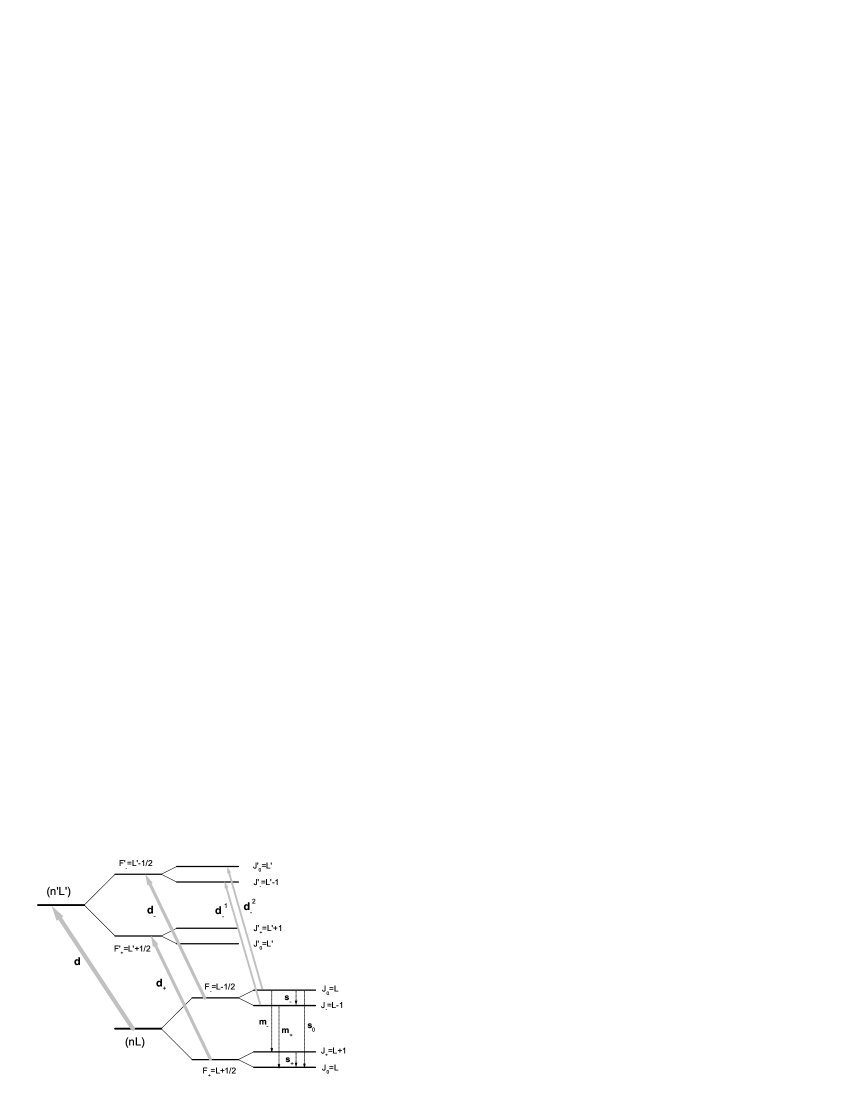
Figure 1: Hyperfine structure of a pair of parent and daughter states of ${\bar{p}}^{4}\!$He and of the dipole transition $(nL)\rightarrow(n^{\prime}L^{\prime})$ between them. The transitions between states of the $F_{-}$ and $F_{+}$ doublets are denoted by $m_{-}$, $m_{+}$ and $m_{0}$ depending on $\Delta J$; the transitions within the $F_{\pm}$ doublets are labelled as $s_{\pm}$. The transitions between homologous doublets of the parent and daughter states are denoted by $d_{\pm}$, and between the homologous components of the doublets - by $d_{\pm}^{1,2}$.

The HFS of the $(37,35)$ state was first observed in 1997 firstobs , when improved resolution allowed for clearly distinguishing two peaks in the profile of the $(37,35)\rightarrow(38,34)$ transition line. The peaks correspond to the $d_{-}$ and $d_{+}$ transitions on Fig.1; at that time the components $d_{\pm}^{1,2}$ could not be resolved, and the remaining non-diagonal components were too strongly suppressed to be observed HFS98 . The first laser spectroscopy study of the HFS of the $(37,35)$ state was performed in 2002 wid-hfs ; using the triple resonance method the frequencies of the $m_{\pm}$ transitions were measured with an accuracy of the order of 300 kHz (below 30 ppm). The idea of the method was to depopulate the $F_{-}$ doublet with a laser pulse tuned at the frequency of the $d_{-}$ transition, then refill it from the $F_{+}$ doublet by applying an oscillating magnetic field tuned at the $m_{-}$ or $m_{+}$ transition frequency, and measure the refilling rate with a repeated laser pulse tuned at the $d_{-}$ transition frequency. In future measurements of the $m_{\pm}$ transition frequencies the experimental uncertainty is expected to be further reduced. In what follows we are analyzing the restrictions that theoretical and experimental uncertainties impose on the value of the antiproton dipole magnetic moment as extracted from spectroscopy data, and outline an alternative approach to improving the accuracy of this value, possibly by up to 2 orders of magnitude.

II Hyperfine structure of the energy levels of the metastable states of ${}^{4\!}$He

The spin interaction Hamiltonian $V$, used in the calculations of the HFS of ${\bar{p}}^{4}\!$He in HFS98 ; HFS01 , has the form of a sum of pairwise interaction terms: $V=V_{\alpha e}+V_{\alpha\bar{p}}+V_{\bar{p}e}$, with (in units $\hbar=e=1$)

$$V_{\alpha e}=\alpha^{2}\left\{\right.\left(1+2\mu_{e}\right){1\over m^{2}_{e}r_{\alpha e}^{3}}(\mathbf{r}_{\alpha e}\times\mathbf{p}_{e})\cdot\mathbf{s}_{e}-{2\mu_{e}\over m_{e}m_{\alpha}r_{\alpha e}^{3}}(\mathbf{r}_{\alpha e}\times\mathbf{p}_{\alpha})\cdot\mathbf{s}_{e}\left.\right\}$$ (1)

$$V_{\alpha\bar{p}}=\alpha^{2}\left\{\right.\left(1+2\mu_{\bar{p}}\right){1\over m^{2}_{\bar{p}}r_{\alpha\bar{p}}^{3}}(\mathbf{r}_{\alpha\bar{p}}\times\mathbf{p}_{\bar{p}})\cdot\mathbf{s}_{\bar{p}}-{2\mu_{\bar{p}}\over m_{\bar{p}}m_{\alpha}r_{\alpha\bar{p}}^{3}}(\mathbf{r}_{\alpha\bar{p}}\times\mathbf{p}_{\alpha})\cdot\mathbf{s}_{\bar{p}}\left.\right\}$$ (2)

$$V_{\bar{p}e}=\alpha^{2}\left\{\right.-\frac{8\pi}{3}\,\frac{\mu_{\bar{p}}\,\mu_{e}}{m_{\bar{p}}\,m_{e}}(\mathbf{s}_{\bar{p}}\cdot\mathbf{s}_{e})\,\delta(\mathbf{r}_{\bar{p}e})-{1\over r^{5}_{\bar{p}e}}\frac{\mu_{\bar{p}}\,\mu_{e}}{m_{\bar{p}}\,m_{e}}\left(3(\mathbf{r}_{\bar{p}e}\cdot\mathbf{s}_{\bar{p}})(\mathbf{r}_{\bar{p}e}\cdot\mathbf{s}_{e})-r_{\bar{p}e}^{2}(\mathbf{s}_{\bar{p}}\cdot\mathbf{s}_{e})\right)$$

$$-\left(1+2\mu_{\bar{p}}\right){1\over 2m^{2}_{\bar{p}}r_{\bar{p}e}^{3}}(\mathbf{r}_{\bar{p}e}\times\mathbf{p}_{\bar{p}})\cdot\mathbf{s}_{\bar{p}}-{\mu_{e}\over m_{\bar{p}}m_{e}r_{\bar{p}e}^{3}}(\mathbf{r}_{\bar{p}e}\times\mathbf{p}_{\bar{p}})\cdot\mathbf{s}_{e}$$

$$+\left(1+2\mu_{e}\right){1\over 2m^{2}_{e}r_{\bar{p}e}^{3}}(\mathbf{r}_{\bar{p}e}\times\mathbf{p}_{e})\cdot\mathbf{s}_{e}+{\mu_{\bar{p}}\over m_{\bar{p}}m_{e}r_{\bar{p}e}^{3}}(\mathbf{r}\times\mathbf{p}_{e})\cdot\mathbf{s}_{\bar{p}}\left.\right\}$$ (3)

Here $m_{i}$, $\mathbf{r}_{i}$, $\mathbf{p}_{i}$ and $\mathbf{s}_{i}$, $i=e,\bar{p},\alpha$ stand for the mass, position vector, momentum and spin operator of the $i$-th constituent of the ${\bar{p}}^{4}\!$He atom, $\mathbf{r}_{ij}=\mathbf{r}_{j}-\mathbf{r}_{i}$. and $\mu_{i}$ is the magnetic moment of particle $i$ in units of “own magnetons” $|e_{i}|\hbar/2m_{i}\equiv 1/2m_{i}$, $e_{i}$ being the electric charge in units $e$. In first order of perturbation theory the hyperfine energy levels $E_{nLFJ}$ are calculated as eigenvalues of the matrix of $V$ in an appropriate basis. The computational procedure makes use of the effective spin Hamiltonian of the system – a finite-dimensional operator acting in the space of the spin and orbital momentum variables of the particles:

$$H_{\text{eff}}\!=\!H_{1}\,(\mathbf{s}_{e}\cdot\mathbf{L})+H_{2}\,(\mathbf{s}_{\bar{p}}\cdot\mathbf{L})+H_{3}\,(\mathbf{s}_{\bar{p}}\cdot\mathbf{s}_{e})+H_{4}\,(2L(L+1)(\mathbf{s}_{\bar{p}}\cdot\mathbf{s}_{e})-3((\mathbf{s}_{\bar{p}}\cdot\mathbf{L})(\mathbf{s}_{e}\cdot\mathbf{L})+(\mathbf{s}_{e}\cdot\mathbf{L})(\mathbf{s}_{\bar{p}}\cdot\mathbf{L}))).$$ (4)

The coefficients $H_{i},i=1,\ldots,4$ of $H_{\rm eff}$ are calculated by averaging the spin interaction Hamiltonian $V$ of Eqs. (1)-(3) with the non-relativistic three-body wave functions of ${\bar{p}}^{4}\!$He; the remaining part of the computations is reduced to angular momentum algebra. The uncertainty of $V$ is determined by the contribution of the interaction terms of order $O(m_{e}\alpha^{6})$ and higher, that have not been taken into consideration. Accordingly, the relative uncertainty $\Delta_{\rm q}H_{i}$ of the coefficients $H_{i}$, due to truncating the expansion of $V$ in power series in $\alpha$ is estimated to be of relative order $\Delta_{\rm q}H_{i}\sim O(\alpha^{2})\sim 10^{-4}$ HFS98 ; HFS01 . The uncertainty of $H_{i}$ gives rise to the uncertainties $\delta_{\rm q}E_{nLFJ}$ and $\delta_{\rm q}\nu$ of the hyperfine energy levels and the hyperfine transition frequencies, respectively, and to the relative uncertainties $\Delta_{\rm q}E_{nLFJ}=\delta_{\rm q}E_{nLFJ}/E_{nLFJ}$ and $\Delta_{\rm q}\nu=\delta_{\rm q}\nu/\nu$. The latter are expressed in terms of the response of $E_{nLFJ}$ and $\nu$ to variations of $H_{i}$ around the values calculated with the spin interaction Hamiltonian $V$, and are given by the derivatives $R_{i}(FJ)=\partial\Delta_{\rm q}E_{nLFJ}/\partial\Delta_{\rm q}H_{i}|_{\Delta_{\rm q}H_{i}=0}$ and $R_{i}(\nu)=\partial\Delta_{\rm q}\nu/\partial\Delta_{\rm q}H_{i}|_{\Delta_{\rm q}H_{i}=0}$. Table 1, presenting the numerical values of these derivatives for the hyperfine levels of the $(37,35)$ state, shows that the theoretical accuracy for all five allowed hyperfine transitions is of the order of $\Delta_{\rm q}H_{i}\sim 10^{-4}$ since $|R_{i}|$ does not exceed 1 and no precision is lost. We have also included in consideration the difference $X$ of the transition frequencies of the $m_{-}$ and $m_{+}$ transitions, $X=\nu(m_{-})-\nu(m_{+})$. This combination is of interest because, on the one hand, it is quite sensitive to the value of $\mu_{\bar{p}}$, and on the other, an improvement of the precision on the $m_{-}$ and $m_{+}$ transition frequencies and therefore also on $X$ by at least one order of magnitude is expected in experiments using an improved laser system in the near future ASACUSAprop .

Table 1: Response of the hyperfine energy levels $E_{nLFJ}$, of the hyperfine transition frequencies $\nu$ and of the difference $X$ of the $m_{-}$ and $m_{+}$ transition frequencies in the metastable state $(37,35)$ of the ${\bar{p}}^{4}\!$He atom to variations of the effective spin Hamiltonian coefficients $H_{i}$. Listed are the dimensionless derivatives $\partial\Delta_{\rm q}E_{nLFJ}/\partial\Delta_{\rm q}H_{i}$ and $\partial\Delta_{\rm q}\nu/\partial\Delta_{\rm q}H_{i}$, evaluated numerically at $\Delta_{\rm q}H_{i}=0$, i.e. using the values calculated with the spin interaction Hamiltonian $V$.

$i$	$R(F_{-}J_{0})$	$R(F_{-}J_{-})$	$R(F_{+}J_{+})$	$R(F_{+}J_{0})$	$R(s_{-})$	$R(s_{+})$	$R(m_{-})$	$R(m_{+})$	$R(m_{0})$	$R(X)$
1	1.010	0.989	0.986	1.012	$-$0.031	$-$0.025	0.998	1.000	0.988	0.000
2	$-$0.012	0.011	0.012	$-$0.012	1.125	0.929	0.000	0.000	0.011	0.000
3	$-$0.011	0.012	$-$0.011	0.012	1.141	$-$0.903	$-$0.011	0.012	0.000	$-$10.613
4	0.013	$-$0.012	0.013	$-$0.012	$-$1.235	0.999	0.013	$-$0.012	0.000	11.613

Note that the theoretical prediction for $X$ is less accurate than for the 5 hyperfine transition frequencies. The uncertainty of the value of $X$, $\Delta_{\rm q}(X)=\max_{i}\,|R_{i}(X).\Delta_{\rm q}H_{i}|$, is larger than $10^{-4}$ and is strongly state-dependent (see Table 2). The values in the table were calculated with the assumption that the uncertainties of $H_{i},i=1,\ldots,4$ are not correlated, and should be regarded as upper limits for the theoretical uncertainties of $X$.

Table 2: Relative uncertainty $\Delta_{\rm q}(X)$ of the theoretical value of the frequency $X$ in the metastable states of the ${\bar{p}}^{4}\!$He atom, due to neglecting the higher-order terms in the spin interaction Hamiltonian $V$ of Eqs. (1)-(3).

$(n,L)$	$(35,33)$	$(37,34)$	$(39,35)$	$(33,32)$	$(36,34)$	$(37,35)$	$(35,34)$	$(34,33)$	$(38,35)$
$\Delta_{\rm q}(X)$	$6\times 10^{-4}$	$11\times 10^{-4}$	$3\times 10^{-4}$	$8\times 10^{-4}$	$23\times 10^{-4}$	$12\times 10^{-4}$	$6\times 10^{-4}$	$4\times 10^{-4}$	$5\times 10^{-4}$

The dominating contribution to $E_{nLFJ}$ comes from the electron spin–orbit interaction which does not depend of the value of the dipole magnetic moment of the antiproton. The value of $\mu_{\bar{p}}$ may be determined from spectroscopy data about the HFS of ${\bar{p}}^{4}\!$He if one selects hyperfine transitions whose frequencies depend as strongly as possible on the value of $\mu_{\bar{p}}$. To help making the appropriate choice, we calculate - for the 9 metastable states that have been experimentally observed by now - the “sensitivity” of the hyperfine levels $E_{nLFJ}$ and of the transition frequencies between them to variations of $\mu_{\bar{p}}$ around the CPT-prescribed value $\mu_{\bar{p}}=-\mu_{p}$. (In agreement with gabrielse we neglect the effects of the small difference of less than $10^{-10}$ between the “own magnetons ” of the proton and antiproton). We define the sensitivity $S(FJ)\equiv S(nLFJ)$ of the hyperfine level $E_{nLFJ}$ as:

$$S(FJ)=\partial E_{nLFJ}/\partial\mu_{\bar{p}}|_{\mu_{\bar{p}}=-\mu_{p}}$$ (5)

The sensitivity of a transition frequency is then the difference of the sensitivities of the initial and final states, e.g. $S(s_{-})=S(F_{-}J_{0})-S(F_{-}J_{-})$, $S(m_{0})=S(F_{-}J_{0})-S(F_{+}J_{0})$, etc. The sensitivity values in Table 3 have been calculated by numerical differentiation of the eigenvalues $E_{nLFJ}$ of the spin interaction Hamiltonian. Because of the opposite signs of $S$ for the upper and lower sublevels in the $F_{-}$ and $F_{+}$ doublets, the sensitivity of the $s_{-}$, $s_{+}$ and $m_{0}$ hyperfine transitions is enhanced, while the sensitivity of the $m_{-}$ and $m_{+}$ transitions is suppressed by orders(s) of magnitude (see Fig. 1).

Table 3: Sensitivities $S(FJ)$ of the hyperfine sublevels from the HFS of a selection of metastable states of the ${\bar{p}}^{4}\!$He atom to variations of the magnetic moment of the antiproton, and sensitivities $S$ of the hyperfine transitions between these sublevels (see Fig. 1) and of the difference $X=\nu(m_{-})-\nu(m_{+})$, in units MHz.

$(nL)$	$S(F_{-}J_{0})$	$S(F_{-}J_{-})$	$S(F_{+}J_{+})$	$S(F_{+}J_{0})$	$S(s_{-})$	$S(s_{+})$	$S(m_{-})$	$S(m_{+})$	$S(m_{0})$	$S(X)$
$(35,33)$	$-$52.6	54.8	$-$45.5	40.5	$-$107.4	$-$86.0	$-$7.1	14.2	100.2	$-$21.3
$(37,34)$	$-$30.6	32.6	$-$38.9	34.9	$-$63.2	$-$73.8	8.4	$-$2.3	71.5	10.7
$(39,35)$	$-$15.0	16.9	$-$33.7	30.6	$-$31.9	$-$64.4	18.8	$-$13.7	50.6	32.5
$(33,32)$	$-$81.8	83.9	$-$55.3	49.2	$-$165.6	$-$104.5	$-$26.4	34.6	139.2	$-$61.1
$(36,34)$	$-$39.5	41.7	$-$40.2	35.8	$-$81.2	$-$76.0	0.7	5.8	81.8	$-$5.1
$(37,35)$	$-$28.2	30.3	$-$36.2	32.3	$-$58.5	$-$68.5	8.0	$-$2.1	66.5	10.1
$(35,34)$	$-$50.1	52.3	$-$41.3	36.5	$-$102.4	$-$77.9	$-$8.7	15.8	93.7	$-24.5$
$(34,33)$	$-$64.8	67.0	$-$47.3	41.9	$-$131.9	$-$89.2	$-$17.5	25.1	114.4	$-$42.6
$(38,35)$	$-$20.8	22.8	$-$35.1	31.7	$-$43.7	$-$66.8	14.3	$-$8.8	57.9	23.1

The current uncertainty in the value of the magnetic moment of the antiproton $\delta\mu_{\bar{p}}\sim 3.10^{-3}\times\mu_{\bar{p}}\sim 8.10^{-3}$ gives rise to an uncertainty $\delta_{\mu}\nu$ of the theoretical frequency $\nu$ of the various hyperfine transitions, that is expressed in terms of the sensitivity $S$: $\delta_{\mu}\nu=|S|.\delta\mu_{\bar{p}}$. The corresponding relative uncertainty $\Delta_{\mu}\nu$ is given by $\Delta_{\mu}\nu=\delta_{\mu}\nu/\nu$. A measurement of the frequency $\nu$ of a hyperfine transition with an experimental uncertainty $\delta_{\rm exp}\nu$ could improve the current accuracy of the antiprotonic magnetic moment value only if (1) the experimental error is sufficiently smaller than the theoretical uncertainties $\delta_{\mu}\nu$ and $\delta_{\rm q}\nu$, and (2) $\delta_{\rm q}\nu<\delta_{\mu}\nu$ or, equivalently, $\Delta_{\mu}\nu/\Delta_{\rm q}\nu>1$. Table 4 presents the value of the absolute uncertainty $|\delta_{\mu}\nu|$ and of the ratio $|\Delta_{\mu}\nu/\Delta\nu_{\rm q}|$ for all hyperfine transitions in the nine observed metastable states of the ${\bar{p}}^{4}\!$He atom. In absence of more precise theoretical calculation which take consistently into account all QED and relativistic effects of order $O(m_{e}\alpha^{6})$, we have assumed (in agreement with the results in Table 1) that $\Delta_{\rm q}\nu=10^{-4}$ for all hyperfine transitions. For the difference $X$ of the $m_{-}$ and $m_{+}$ transition frequencies we used the values of $\Delta_{\rm q}(X)$ from Table 2.

Table 4: Absolute uncertainty $\delta_{\mu}\nu$ (in MHz), related to the current uncertainty of 0.3% of the magnetic dipole moment of the antiproton, and the ratio $\Delta_{\mu}\nu/\Delta_{q}\nu$ of the relative theoretical uncertainties $\Delta_{\mu}\nu$ and $\Delta_{q}\nu$ of the hyperfine transition frequencies in the metastable states $(nL)$ of ${\bar{p}}^{4}\!$He. For the labelling of the hyperfine transitions, see Fig. 1; $X$ labels the difference of the $m_{-}$ and $m_{+}$ transition frequencies.

$(nL)$		$s_{-}$	$s_{+}$	$m_{-}$	$m_{+}$	$m_{0}$	$X$
$(35,33)$	$\delta_{\mu}\nu$	$0.90$	$0.72$	$0.06$	$0.12$	$0.84$	$0.18$
	$\Delta_{\mu}\nu/\Delta_{\rm q}\nu$	$35.3$	$36.9$	$0.0$	$0.1$	$0.6$	$5.0$
$(37,34)$	$\delta_{\mu}\nu$	$0.53$	$0.62$	$0.07$	$0.02$	$0.60$	$0.09$
	$\Delta_{\mu}\nu/\Delta_{\rm q}\nu$	$36.8$	$35.6$	$0.1$	$0.0$	$0.6$	$2.7$
$(39,35)$	$\delta_{\mu}\nu$	$0.27$	$0.54$	$0.16$	$0.11$	$0.42$	$0.27$
	$\Delta_{\mu}\nu/\Delta_{\rm q}\nu$	$40.6$	$34.4$	$0.1$	$0.1$	$0.4$	$8.9$
$(33,32)$	$\delta_{\mu}\nu$	$1.39$	$0.88$	$0.22$	$0.29$	$1.17$	$0.51$
	$\Delta_{\mu}\nu/\Delta_{\rm q}\nu$	$34.6$	$38.0$	$0.1$	$0.2$	$0.8$	$3.6$
$(36,34)$	$\delta_{\mu}\nu$	$0.68$	$0.64$	$0.00$	$0.05$	$0.69$	$0.05$
	$\Delta_{\mu}\nu/\Delta_{\rm q}\nu$	$35.9$	$36.3$	$0.0$	$0.0$	$0.5$	$1.3$
$(37,35)$	$\delta_{\mu}\nu$	$0.49$	$0.57$	$0.07$	$0.02$	$0.56$	$0.09$
	$\Delta_{\mu}\nu/\Delta_{\rm q}\nu$	$36.9$	$35.7$	$0.1$	$0.0$	$0.4$	$2.7$
$(35,34)$	$\delta_{\mu}\nu$	$0.86$	$0.65$	$0.07$	$0.13$	$0.79$	$0.21$
	$\Delta_{\mu}\nu/\Delta_{\rm q}\nu$	$35.3$	$37.1$	$0.0$	$0.1$	$0.5$	$5.4$
$(34,33)$	$\delta_{\mu}\nu$	$1.11$	$0.75$	$0.15$	$0.21$	$0.96$	$0.36$
	$\Delta_{\mu}\nu/\Delta_{\rm q}\nu$	$35.0$	$37.9$	$0.1$	$0.1$	$0.6$	$8.4$
$(38,35)$	$\delta_{\mu}\nu$	$0.37$	$0.56$	$0.12$	$0.07$	$0.49$	$0.19$
	$\Delta_{\mu}\nu/\Delta_{\rm q}\nu$	$38.8$	$35.0$	$0.1$	$0.1$	$0.4$	$6.0$

To improve the current accuracy of 0.3% of $\mu_{\bar{p}}$, the absolute experimental uncertainty $\delta_{\rm exp}\nu$ of the measurement of the transition frequency $\nu$ should be below the corresponding value $\delta_{\mu}\nu$ of Table 4. Provided that this condition is fulfilled, the ratio $\Delta_{\mu}\nu/\Delta_{\rm q}\nu$ is an estimate of the expected factor of improvement of the accuracy of $\mu_{\bar{p}}$. In other words, the ratio $\Delta_{\mu}\nu/\Delta\nu_{\rm q}$ is a criterium for selecting the hyperfine transitions that are most appropriate for determining $\mu_{\bar{p}}$. A quick look at the Table 4 shows that measurements of the $s_{-}$ and $s_{+}$ transitions in any of the metastable states would improve the accuracy of the experimental values of $\mu_{\bar{p}}$ by a factor between 35 and 40. Measurements of the difference $X$ of $m_{-}$ and $m_{+}$ transition frequencies in the $(39,35)$ and $(34,33)$ states might improve the value of $\mu_{\bar{p}}$ by an order of magnitude. No gain of accuracy is expected from measurements of the $m_{\pm}$ and $m_{0}$ transitions.

III Application of the triple resonance method to measurements of the hyperfine transition frequencies

The $s_{-}$ and $s_{+}$ transition frequencies could be measured using an analog of the triple resonance method of Ref. wid-hfs . Initially, the $J_{-}$ and $J_{0}$ sublevels of the $F_{-}$ doublet (see Fig. 1) are equally populated. By applying a laser pulse, tuned at the resonance frequency of the $d_{-}^{1}$ transition and de-tuned from the $d_{-}^{2}$ frequency, the $J_{-}$ and $J_{0}$ sublevels are depopulated asymmetrically. Symmetry is (partially) restored by resonance magnetic field-stimulated $s_{-}$ transitions. The fulfillment of the resonance condition is checked by means of a second, delayed laser pulse of the same frequency as the first one, intended to display any increase of the population of the $J_{-}$ sublevel. The expected difficulties in such a measurement are related to the low intensity of the $s_{\pm}$ transition lines and to the overlap of the $d_{-}^{1,2}$ transition line profiles that makes the efficiency of the asymmetrical depopulation of the $F_{-}$ doublet far from obvious.

The $s_{-}$, $s_{+}$ and $m_{0}$ transition lines are much weaker than the $m_{-}$ and $m_{+}$ lines, which were subject to spectroscopy measurements by the ASACUSA collaboration in 2002 wid-hfs . Compared to the Rabi frequency $\nu_{R}$ of $m_{-}$ and $m_{+}$, $\nu_{R}(m_{\pm})\approx(\mu_{B}B_{0})/\sqrt{6}$, the Rabi frequencies of $s_{\pm}$ and $m_{0}$ are suppressed by factors of the order of $L$: $\nu_{R}(m_{0})/\nu_{R}(m_{\pm})\sim(1+2\phi L)/L\sqrt{2}$, $\nu_{R}(s_{\pm})/\nu_{R}(m_{\pm})\sim(1+2\phi L)/2L$, where $\phi\sim 2.10^{-2}$ is the mixing angle of the $F_{\pm}$ components in the $J=L$ hyperfine states (see Table II of Ref. HFS98 ). Precision spectroscopy of the $s_{-}$ and $s_{+}$ transition lines would therefore require a longer measurement time and a stronger magnetic field, oscillating with frequencies in the 100 – 200 MHz range.

Figure 2: Asymmetric depopulation of the hyperfine states $J_{-}$ and $J_{0}$ of the $F_{-}$ doublet.

To estimate the efficiency of asymmetrical depopulation, we consider a simple model in which the laser line profile is assumed to be a Gaussian, centered at $\nu_{\rm las}$: $\rho_{\rm las}(\nu;\nu_{\rm las},w_{\rm las})=(w_{\rm las}\sqrt{\pi})^{-1}\exp(-(\nu-\nu_{\rm las})^{2}/w_{\rm las}^{2})$, while the profiles of the $d_{-}^{i}$ transition lines are assumed to be Voigtian (i.e. convolutions of a Gaussian and a Lorenzian), centered at $\nu_{i},i\!=\!1,2$ (see Fig.2): $\rho_{i}(\nu;\nu_{i},w_{D},\Gamma_{c})=(w_{D}\sqrt{\pi})^{-1}K(\nu/w_{D},\Gamma_{c}/w_{D})$, where the definition and computational algorithms for the Voigt function $K(x,y)$ may be found in voigt3 , $\Gamma_{c}$ is the collisional HWHM width of the $d_{-}^{1,2}$ transition lines, and the parameters $w_{\rm las}$ and $w_{D}$ are related to the FWHM width $\Gamma_{\rm las}$ of the laser profile and the Doppler width $\Gamma_{D}$ of the $d_{-}^{1,2}$ lines by means of $w_{\rm las}=\Gamma_{\rm las}/2\sqrt{\,\log 2}$, and similar for $w_{D}$. The depopulation rates of the $J_{-}$ and $J_{0}$ sublevels, $\lambda_{1,2}$, are proportional to the overlap of the laser line profile with the profiles of the $d_{-}^{1,2}$ transition lines: $\lambda_{i}(\nu_{i}\!-\!\nu_{\rm las})={\rm const}.\int d\nu\,\rho_{\rm las}(\nu;\nu_{\rm las},w_{\rm las})\,\rho_{i}(\nu;\nu_{i},w_{d},\Gamma_{c})$, where the dependence on the detuning $(\nu_{i}-\nu_{\rm las})$ has been displayed explicitly. Denote by $d$ the distance between the $d_{-}^{1}$ and $d_{-}^{2}$ transition frequencies: $d=\nu_{1}-\nu_{2}$, and by $D=(\nu_{\rm las}-\nu_{1})$ – the detuning between $\nu_{1}$ and $\nu_{\rm las}$ (see Fig. 2). The depopulation asymmetry is described with the ratio of the rates of depopulation of the $J_{-}$ and $J_{0}$ states $q(D)=\lambda_{1}(D)/\lambda_{2}(D+d)$. The depopulation rate $\lambda_{1}$ may be arranged to exceed $\lambda_{2}$ by the factor $q>1$ by choosing the detuning $D$ to satisfy the nonlinear equation $q(D)=q$. This equation has real solutions only for $q$ in the range $1\leq q\leq q_{\rm max}$, with different $q_{\rm max}$ for each transition depending on the values of $\Gamma_{c}$, $\Gamma_{d}$ and $\Gamma_{\rm las}$. The price for the achieved asymmetry will be a smaller overlap of the $\rho_{\rm las}$ and $\rho_{1}$ profiles, and, as a consequence – waste of laser power and lower $\lambda_{1}$ rate. The waste of laser power may be described in terms of the “power loss factor” $f=f(D)$, defined as

$$f\!\equiv\!f(D)=\!\int d\nu\,\rho_{1}(\nu;0,w_{d},\Gamma_{c})\,\rho_{\rm las}(\nu;D,w_{\rm las})\,\big{/}\!\int d\nu\,\rho_{1}(\nu;0,w_{d},\Gamma_{c})\,\rho_{\rm las}(\nu;0,w_{\rm las}).$$ (6)

To get a quantitative idea of the discussed phenomena, we calculate – for all ten transitions in consideration – the values of the detuning $D$ that lead to asymmetrical depopulation rates ratio $q=1.2$ and $q=1.5$ (if these values are within the range $[1,q_{\rm max}]$), as well as the related power loss factor $f$, using the realistic value 100 MHz for the FWHM of the laser profile current . The collisional HWHM widths $\Gamma_{c}$ were calculated for temperature $T=6^{\circ}K$ and helium gas target number density $3\times 10^{20}\ cm^{-3}$ using the results of Ref. prl2k . The numerical results are presented in Table 5.

Table 5: Values of the detuning $D$ (in MHz) of the frequency $\nu_{\rm las}$ of the depopulating laser, reckoned from the frequency $\nu_{1}$ of the dipole transitions $d^{1}_{-}$ from the $F_{-}$ hyperfine doublet, that lead to asymmetric depopulation of the doublet hyperfine states with a depopulation rate ratio $q=120$% and $q=150$%. The space is left empty when $q$ exceeds the maximal accessible values $q_{\rm max}$ for the transition. Also listed are the associates laser power loss factors $f$.

asymmetric depopulation rate ratio $q$						120%		150%
$(nL)\rightarrow(n^{\prime}L^{\prime})$	$\lambda$ (nm)	$\Gamma_{c}$ (MHz)	$\Gamma_{d}$ (MHz)	$d$ (MHz)	$q_{\rm max}$	$D$ (MHz)	$f$	$D$ (MHz)	$f$
$(39,35)\rightarrow(38,34)$	597	108	393	40.9	1.26	218	0.62
$(37,34)\rightarrow(36,33)$	470	24	499	57.1	1.62	136	0.84	359	0.29
$(35,33)\rightarrow(34,32)$	372	9	630	75.1	1.92	146	0.87	375	0.39
$(33,32)\rightarrow(32,31)$	296	6	792	77.9	1.81	234	0.79	575	0.24
$(37,35)\rightarrow(38,34)$	726	75	323	26.3	1.21	247	0.40
$(36,34)\rightarrow(37,33)$	617	33	380	33.9	1.37	163	0.66
$(37,34)\rightarrow(38,33)$	714	90	328	25.0	1.18
$(35,34)\rightarrow(36,33)$	533	15	440	42.5	1.55	148	0.76	387	0.16
$(34,33)\rightarrow(35,32)$	458	9	512	48.5	1.54	167	0.76	416	0.18
$(38,35)\rightarrow(39,34)$	842	183	278	18.5	1.09

IV Conclusions

We have shown that high accuracy measurements of appropriate hyperfine transition lines in the metastable states of antiprotonic helium can help reduce the experimental uncertainty of the dipole magnetic moment of the antiproton. An improvement of the current experiment measuring the $m_{+}$, $m_{-}$ and as a consequence $X$, is being prepared and it is expected to improve the accuracy on $\mu_{\bar{p}}$ by up to a factor of 9. A larger improvement by a factor of up to 40 is possible by directly measuring the antiproton spin-flip transitions $s_{+}$ and $s_{-}$. The restrictions on the expected gain of accuracy come from the difficulty to reduce the experimental uncertainty below the threshold $\delta_{\mu}\nu$ in Table 4 rather than from the limited accuracy of the Breit spin interaction Hamiltonian $V$ of Eqs. (1)-(3) used in the theoretical calculations. We have also outlined a possible experimental method for the measurement of the super-hyperfine splitting, without discussing in details the feasibility of the experiment. We leave for future works the numerical simulations that will answer questions about the restrictions on the experimental accuracy from the expectedly rather low signal-to-noise ratio and about the possible use of a large oscillatory magnetic filed in cryogenic helium gas target.

The authors express their gratitude to Dr. V.I.Korobov for the many fruitful discussions on the subject.

References

- (1) J.Eades and F.J.Hartmann, Rev. Mod. Phys. 71, 373 (1999).
- (2) T. Yamazaki, N. Morita, R. S. Hayano, E. Widmann, and J. Eades, Phys. Rep. 366, 183 (2002).
- (3) M. Hori et al., Phys. Rev. Lett. 96, 243401 (2006).
- (4) S.G. Karshenboim, Int. J. Mod. Phys. A19, 3879 (2004).
- (5) G. S. Adkins, R. N. Fell, and P. Mitrikov, Phys. Rev. Lett. 79, 3383 (1997); A. H. Hoang, P. Labelle, and S. M. Zebarjad, Phys. Rev. Lett. 79, 3387 (1997).
- (6) M.W. Ritter, P.O. Egan, V.W. Hughes, and K.A. Woodle, Phys. Rev. A 30, 1331 (1984).
- (7) A. Kreissl et al., Z. Phys. C 37, 557 (1988)
- (8) D.Bakalov, V.I.Korobov, Phys. Rev. A 57, 1662 (1998).
- (9) V.I.Korobov and D.Bakalov, J. Phys. B34, L519 (2001).
- (10) P.J. Mohr and B.N. Taylor, Rev. Mod. Phys. 77, 1 (2005).
- (11) G.T.Condo, Phys. Lett. 9, 65 (1964).
- (12) E.Widmann et al., Phys. Lett. B 404, 15 (1997).
- (13) ASACUSA proposal CERN/SPSC 2005-002 (2005).
- (14) G. Gabrielse et al., Phys. Rev. Lett. 82, 3198 (1999).
- (15) E.Widmann et al., Phys. Rev. Lett. 89, 243402 (2002).
- (16) J.H. Pierluissi, P.C. Vanderwood, and R.B. Gomez, J. Quant. Radiat. Transfer, 18, 555 (1977).
- (17) M. Hori et al. Phys. Rev. Lett. 96, 243401 (2006).
- (18) D. Bakalov, B. Jeziorski, T. Korona, K. Szalewicz, and E. Tchukova, Phys. Rev. Lett. 84, 2350 (2000).