Relaxation and phase space singularities in time series of human magnetoencephalograms as indicator of photosensitive epilepsy

Abstract

To analyze the crucial role of fluctuation and relaxation effects for the function of the human brain we studied some statistical quantifiers that support the information characteristics of neuromagnetic brain responses (magnetoencephalogram, MEG). The signals to a flickering stimulus of different color combinations have been obtained from a group of control subjects which is then contrasted with those of a patient suffering photosensitive epilepsy (PSE). We found that the existence of the specific stratification of the phase clouds and the concomitant relaxation singularities of the corresponding nonequilibrium dynamics of the chaotic behavior of the signals in separate areas in a patient provide likely indicators for the zones which are responsible for the appearance of PSE.

I Introduction

The study of dynamical time series is gaining ever increasing interest and is applied and used in diversified fields of natural sciences, technology, physiology, medicine and economics Jade ; Barb ; Rag ; Mar ; Lau ; Hir ; Lau2 ; kantzschreiber , to name only a few. The majority of natural systems can be considered dynamical systems, whose evolution can be studied by time series related to relevant variables on a suitable time scale. These series are often characterized by a pronounced time and spatial synchronization or coherence, chaotic or robust behavior.

When analyzing time series data with linear methods, one can follow certain standard procedures. Moreover, the behavior may be described by a relatively small set of parameters. For a nonlinear time series analysis, this is not necessarily the case. While standardized algorithms exist for the analysis of the time series data with nonlinear methods, the application of these algorithms requires considerable knowledge and skills on the part of the user.

In a nonlinear time series analysis one starts out with a reconstruction of the state spaces from the observed data kantzschreiber ; Tak ; Sau ; Stark ; Sau2 . Although the embedding theorems Schrei provide an important means of understanding the reconstruction procedure, likely none of them is formally applicable in practice. The reason is that they all deal with infinite, noise free trajectories of a dynamical system. It is not obvious that the theorems should be ”approximately valid” if only the requirements are ”approximately fulfilled”, for example, if the data sequence is long, although finite and not completely noise-free.

A possible way to study the manifestation of physical properties of random processes (and the Markov random processes (MRP) in particular) in time series originates from the theory of nonequilibrium statistical physics. The history of the fundamental role of stochastic processes in physics dates back a century to the Markov representations Mark of random telegraphic signals. Such processes still find application in models of contemporary complex phenomena. A few typical examples of complex physical phenomena modeled by the Markov stochastic processes are: kinetic and relaxation processes in gases gases and plasma plasma , condensed matter physics (liquids liq , solids solids , and superconductivity super ), astrophysics astro , nuclear physics nucl , for certain quantum relaxation dynamics quant and in classical class physics. At present, we can make use of a variety of statistical methods for the analysis of the Markov and the non-Markov statistical effects in diverse physical systems. Typical examples of such schemes are the Zwanzig-Mori’s kinetic equations Zwanz , generalized master equations and corresponding statistical quantifiers hanggi , the Lee’s recurrence relation method Lee , the generalized Langevin equation (GLE) GLE , etc.

In this paper we shall study the crucial role of relaxation and kinetic singularities in brain function of healthy physiological and pathological systems for the case of photosensitive epilepsy (PSE). In particular, we seek marked differences in large space and times scales in the corresponding stochastic dynamics of discrete time series that could in principle characterize pathological (or catastrophic) violation of salutary dynamic states of the human brain. As a main result, we show here that the appearance of distinct differences in the relaxation time scales and extraordinary stratification of the phase clouds in the stochastic evolution of neuromagnetic responses of the human brain as recorded by MEG may yield evidence of pronounced zones responsible for the appearance of PSE.

II Stratification in the phase space and stochastic processes in complex systems

The phase space plays a crucial role in determining the singularities of stochastic dynamics of the underlying system. A set of the dynamical orthogonal statistical variables describing the dynamical state of the complex system is a feature important in a proper construction of the phase space and analysis of the underlying dynamics. Let us consider an k-dimensional vector of the initial state ${\bf A}_{k}^{0}=(x_{1},x_{2},x_{3},....x_{k}$) and an k-dimensional dynamic vector of the final state ${\bf A}_{k+m}^{m}=(x_{m+1},x_{m+2},x_{m+3},....x_{m+k}$) , where $k+m=N,k,m=N,N-1,N-2,...,N/2-2,N/2-1,N/2$ and N denotes the sample length. From the discrete equation of motion

$$\frac{\Delta x_{i}}{\Delta t}=\frac{x_{i+1}-x_{i}}{t_{i+1}-t_{i}}=\frac{1}{\tau}\left\{\Delta-1\right\}x_{i},$$

$$t_{i+1}-t_{i}=\tau,$$ (1)

we obtain the equation of motion of the dynamical vectors of state ${\bf A}_{m+k}^{m}$ as:

$$\frac{\Delta{\bf A}_{j}^{m}}{\Delta t}=i\widehat{\emph{L}}A_{j}^{m},$$

$$i\widehat{\emph{L}}=\frac{1}{\tau}{(\Delta-1)}\;,$$ (2)

where the shift operator $\Delta$ acts as $\Delta x_{j}=x_{j+1}$ and j = m+k.

By applying successively the quasioperator $\widehat{\emph{L}}$ to the dynamic variables $A_{j}^{m}(t)$, t=m$\tau,$ where $\tau$ is a discrete time step, $j=m+k$, we obtain the set of dynamic functions ${\bf B}_{n}(0)=\widehat{\emph{L}}^{n}{\bf A}_{k}^{0}(0)$, $n>1$. By using the variables $B_{n}(0)$ one can find a formal solution of the evolution of these equations in the form

$${\bf A}_{m+k}^{m}(m\tau)=\left\{1+i\tau\widehat{\emph{L}}\right\}^{m}{\bf A}_{k}^{0}(0)=\sum_{j=0}^{m}\frac{m!(i\tau)^{m-j}}{j!(m-j)!}{\bf B}_{m-j}^{0}.$$ (3)

However, the use of this structure is generally not the most convenient one. An advantageous approach consists in the use of the orthogonal vectors $W_{n}$, as detailed below, by use of the Gram-Schmidt orthogonalization procedure Reed in place of the set of variables $B_{n}(0)$. Thus, we work with this new set of dynamical orthogonal vector variables, where the average $<...>$ should be read in terms of scalar products and $\delta_{n,m}$ is the Kronecker’s symbol. In doing so, we find the the recurrence formula in which the ”senior” variables at order ”n” $W_{n}=W_{n}(t)$ are related through with the ”junior” variables of order $m<n$; i. e. DFA ; Yulm

$${\bf W}_{0}={\bf A}_{k}^{0}(0),\leavevmode\nobreak\ \leavevmode\nobreak\ {\bf W}_{1}=\{i\hat{L}-\lambda_{1}\}{\bf W}_{0},\ldots\leavevmode\nobreak\ \leavevmode\nobreak\ \\$$

$${\langle{\bf W}_{n}{\bf W}_{m}\rangle}=\delta_{n,m}{\langle|\bf W_{n}|^{2}\rangle},\leavevmode\nobreak\ \leavevmode\nobreak\ \\$$

$${\bf W}_{n}=\{i\hat{L}-\lambda_{n}\}{\bf W}_{n-1}+\Lambda_{n-1}{\bf W}_{n-2}+...,\leavevmode\nobreak\ \leavevmode\nobreak\ n>1.$$ (4)

Here, we have used the kinetic parameters given by the Liouville’s quasioperator L as follows Yulm :

$$\lambda_{n}=\frac{\langle{\bf W_{n}}\widehat{\emph{L}}{\bf W_{n}}\rangle}{\langle|{\bf W_{n}}|^{2}\rangle},$$

$$\Lambda_{n}=\frac{\langle|{\bf W_{n}}|^{2}\rangle}{\langle|{\bf W_{n-1}}|^{2}\rangle},$$ (5)

where $\Lambda_{n}=\Omega_{n-1}^{2}$, with the parameter $\Omega_{n}$ denoting a general relaxation frequency. The set of frequencies $\lambda_{n}$ describes the spectrum of the Liouville’s operator $\widehat{\emph{L}}$.

Besides these relaxation time measures, we in addition shall consider information measures that are based on time correlation functions which assume the role of memory functions $M_{i}(t),i=0,1,2,...$, see in Refs. Yulm ; i. e.,

$$M_{i}(t)=\frac{\langle{\bf W_{i}(0)}{\bf W_{i}(t)}\rangle}{\langle|{\bf W_{i}(0)}|^{2}\rangle}.$$

Note that the quantity with $i=0$ corresponds to the temporal autocorrelation function of the vector ${\bf A}_{k}^{0}$.

III Analysis of time series for the experimental data of PSE

Now we can proceed directly to the analysis of the experimental data: the MEG signals recorded in a group of nine healthy human subjects and a patient with (PSE) MEG . PSE is a common type of stimulus-induced epilepsy, defined as recurrent convulsions precipitated by visual stimuli, particularly flickering light. The diagnosis of PSE involves the detection of paroxysmal spikes on an EEG in response to the intermittent light stimulation. To elucidate the color-dependency of PS in normal subjects, brain activities subjected to uniform chromatic flickers with whole-scalp MEG have been measured in Ref. MEG ).

The same subjects and the data set were part of an earlier study in Ref. MEG ; however, we shall mention the relevant details for the sake of completeness. Nine healthy adults (two females, seven males; with age ranging from 22-27years) voluntarily participated. Two additional age-matched child control subjects, and one more photosensitive patient (age 14yr) under medication (sodium valporate), were also studied. All subjects were right-handed and were explicitly informed that flicker stimulation might lead to epileptic seizures. They gave their written informed consent before recording. The subjects were instructed to passively observe visual stimuli with minimal eye movement. During the testing session for the photosensitive patient, pediatric neurologists were present to monitor their health condition as a precautionary measure.

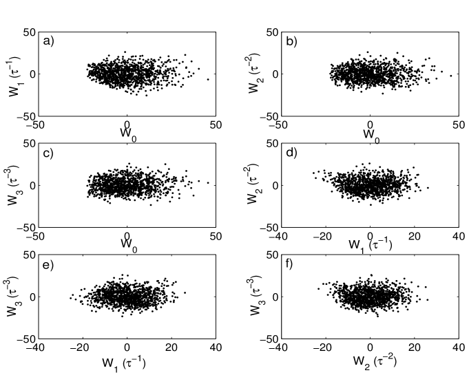
Figure 1: The single phase planes of the phase portrait of the patient with PSE for MEG signals from an R/B combination of the light stimulus : a) plane $(W_{0}(t),W_{1}(t))$; b) plane $(W_{0}(t),W_{2}(t)$); c) plane $(W_{0}(t),W_{3}(t)$); d) plane $(W_{1}(t),W_{2}(t)$); e) plane $(W_{1}(t),W_{3}(t)$); f) plane $(W_{2}(t),W_{3}(t))$.

The subjects were screened for photosensitivity and personal or family history of epilepsy. The experimental procedures followed the Declaration of Helsinki and were approved by the National Children’s Hospital in Japan. The stimuli were generated by the two video projectors and delivered to the viewing window in the shield room through an optical fiber bundle. Each projector continuously produced a single color stimulus. Liquid crystal shutters were located between the optical device and the projectors. By alternative opening one of the shutters for 50 ms, 10 Hz (square-wave) chromatic flicker was produced at the viewing distance of 30 cm. Three color combination were used : red-green (R/G), blue-green (B/G), and red-blue (R/B). CIE coordinates were x=0. 496, y=0. 396 for red; x=0. 308, y=0. 522 for green; and x=0. 153, y= 0. 122 for blue. All color stimuli had the luminance of $1.6$ cd/m² in otherwise total darkness. In a single trial, the stimulus was presented for 2s and followed by an inter-trial interval of 3s, during which no visual stimulus was displayed. In a single session, the color combination was fixed.

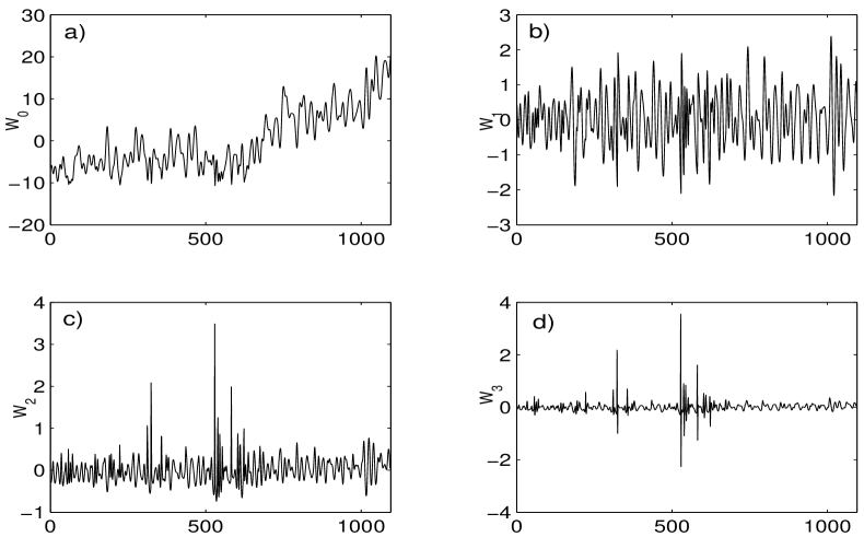
Figure 2: The time dependence of the first four orthogonal variables for MEG signals in healthy in No. 3 ( sensor m = 13, for an R/ B combination of the light stimulus: for healthy subject No. 4 : a) $W_{0}(t)$; b) $W_{1}(t)$; c) $W_{2}(t)$;d) $W_{3}(t)$ for an R/ B combination of the light stimulus.

Neuromagnetic responses were measured with a 122-channel whole-scalp neoromagnetometer (Neuromag - 122; Neuromag Ltd. Finland). The neoromag-122 has 61 sensor locations, each containing two originally oriented planner gradiometers coupled with dc-SCUID (superconducting quantum interference device) sensors. The two sensors of each location measure two orthogonal tangential derivatives of the brain magnetic field component perpendicular to the surface of the sensor array. The planner gradiometers measure the strongest magnetic signals directly above local cortical currents. From 200 ms prior responses were analog-filtered (bandpass frequency 0.03 - 100 Hz) and digitized at 0.5 kHz. Eye movements and blinks were monitored by measuring an electro-oculogram.

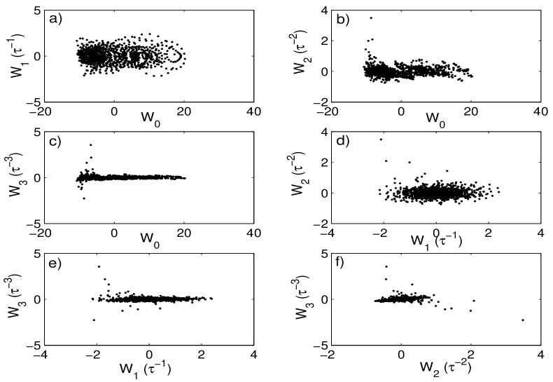
Figure 3: The phase portraits for MEG signals in healthy person No. 3 (sensor number m = 13) for an R/ B combination of the light stimulus. The phase space has been created by the phase points $\Gamma_{i,j}(t)=(W_{i}(t),W_{j}(t)),1\leq i\neq j\leq 3$.

The trials with MEG amplitudes $>3000$ fT/cm and/or electro-oculogram amplitudes $>150\mu$ V were automatically rejected from averaging. The trials were repeated until $>80$ responses were averaged for each color-combination. The averaged MEG signals were digitally lowpass-filtered at 40 Hz, and then the DC offset along the baseline $(-100$ to $0$ ms) was removed. At each sensor location, the magnetic waveform amplitude was calculated as the vector sum of the orthogonal components. The peak amplitude were normalized within each subject with respect to the subject’s maximum amplitude. The latency range from $-100$ to $-1100$ ms was divided into 100 ms bins. Then, the peak amplitudes were calculated by averaging all peak amplitudes within each bin. It would be important to mention that no clinical photosensitive seizures were induced during the experiment. This also confirms the better detection power of this analysis than normal seizure detection procedure.

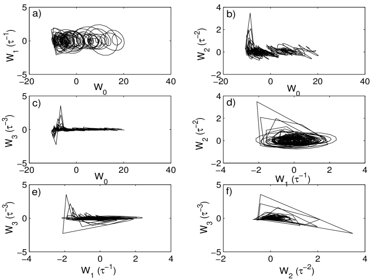
Figure 4: The phase trajectories of the phase points $\Gamma_{i,j}(t)=(W_{i}(t),W_{j}(t))$, healthy person No. 3 (sensor number m = 13) for an R/ B combination of the light stimulus.

IV Results and discussion

Here we present the information-theoretic analysis for the presence of PSE, based on the time behavior of the dynamical variables and the stratified structure of phase spaces. Some results of our quantities as derived from the theory presented here, are depicted in Figs. 1-7. Our results for nine healthy subjects and for the patient with PSE in comparison are shown in Figs. 8 - 10 . Among them are: the time traces of the MEG signals $(W_{0})$, and for the three junior dynamical orthogonal variables $(W_{i})$, i = 1, 2 and 3; 2), the phase space created by the points with coordinates $(W_{i})$, i = 0, 1, 2 and 3; 3) the phase space, filled by the trajectories $(W_{i}(t))$, i = 0, 1, 2 and 3; 4) the time dependence of the first four quantifiers: the time correlation functions (TCF) $M_{0}(t)$ and the first three junior memory functions (MF) $M_{i}(t)$, for i = 1, 2 and 3. The results of the experiment for a red-blue (R/B) and a red-green (R/G) combination of color signals are used in all of the figures.

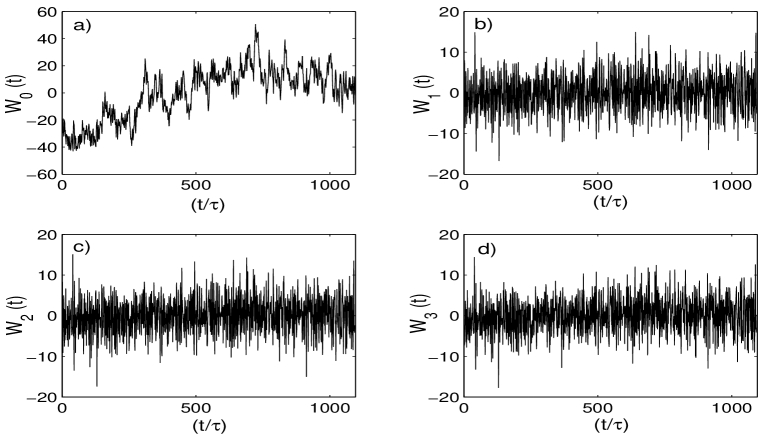
Figure 5: The time dependence of the first four orthogonal variables $W_{i}(t),i=1,2,...3$ for the MEG signals for the patient with PSE, sensor m = 13, an R/ B combination of the light stimulus.

As an example, the analogous results for the patient with PSE(sensor No. 10) are presented in Fig. (1). The obtained results possess the clearly visible inconsistent character. The comparison clearly shows a characteristic behavior of the dynamic variables $(W_{i}(t))$ (i = 1, 2 and 3). The time dependence of the variables $(W_{1}(t))$ presents the time behavior of the orthogonal velocity of the signal recording in discrete form. The next-order dynamic variable $(W_{2}(t))$ describes the orthogonal acceleration, the variable $(W_{3}(t))$ depicts the longitudinal orthogonal energy current, etc. The signals $(W_{i}(t))$ in the patient with PSE can be characterized as regular noise. The phase clouds formed by manifold phase points drastically differ from the healthy ones in comparison with the patient with PSE, see, Fig. 1.

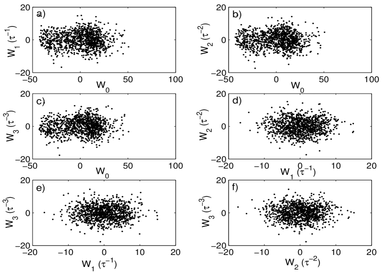
Figure 6: The phase portraits created by the phase points $\Gamma_{i,j}(t)=(W_{i}(t),W_{j}(t))$ from MEG signals for patient with PSE, m = 13, an R/ B combination of the light stimulus.

The stratification of the phase clouds and the existence of the stable pseudoorbits are more visible for the healthy . In the patient with PSE (see,Fig. (1)) the phase stratification disappears. The phase clouds can be characterized by symmetrical nuclei, they have spatial homogeneity. The phase trajectories for the healthy form broken lines.

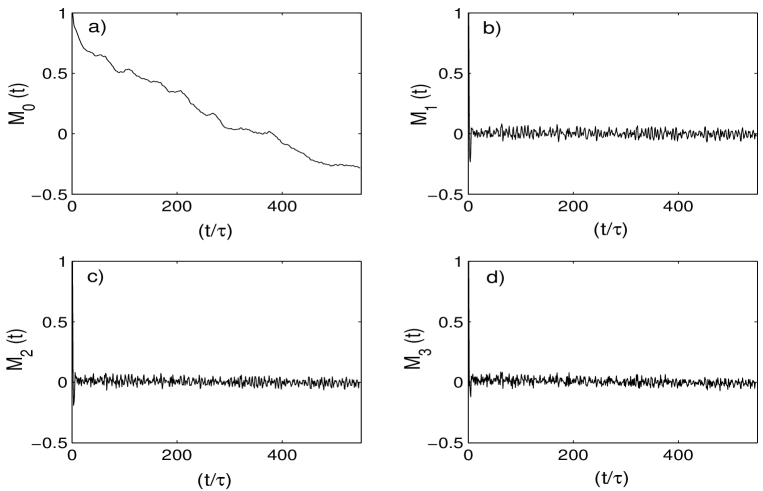
Figure 7: The time dependence of the first four MF’s $M_{i}(t),i=0,1,...3$ for the MEG signals in the patient with PSE ( sensor number m = 13) an R/ B combination of the light stimulus. Large scale fluctuation of all functions become obvious in comparison with a case for the healthy.

For the patient with PSE the pictures of the phase trajectories contrast sharply with the case of the healthy. The phase trajectories are packed tightly within the restricted areas of the phase space. The drastic difference in the typical scales of the dynamic variables $(W_{i}(t))$ and in the size of the phase space for the healthy and for the patient with PSE (Fig. 1) are striking. This difference ranges from 3 times (for $(W_{0}(t))$ ) to 10 times(for $(W_{i}(t)),i=1,2,$ and 3) and from 10 times (for the phase plane ${(W_{0}(t),W_{1}(t)})$ to 80 times in the corresponding clouds of phase planes ${(W_{0}(t),W_{i}(t)})$, i = 2, 3 and ${(W_{i}(t),W_{j}(t)})$ with $1\leq i,j\leq 3$.

Figure 8: The topographic dependence of the first relaxation parameter $\lambda_{1}$ for nine healthy subjects (upper lines) in comparison with the patient with PSE (lower line) for an R/ B combination of the light stimulus. The crucial role of the brain zones with sensor numbers m = 10, 12, 46 , 51 and 53 is clearly visible.

Thus, the signals in the patient with PSE with sensor number 10 differ from the healthy subjects consists in the drastic change of the fluctuation scales of the dynamic orthogonal variables and the space sizes of the phase clouds. The similar difference of the scales constitutes the values from 10 to 80 times. This observation let us note the specific role and behavior of the sensor with number n=10 in the formation of PSE mechanisms! The difference in the scales of the orthogonal dynamic variables and in the sizes of the phase clouds is more drastic for sensors with numbers n = 10, 5, 23, 40 and 53.

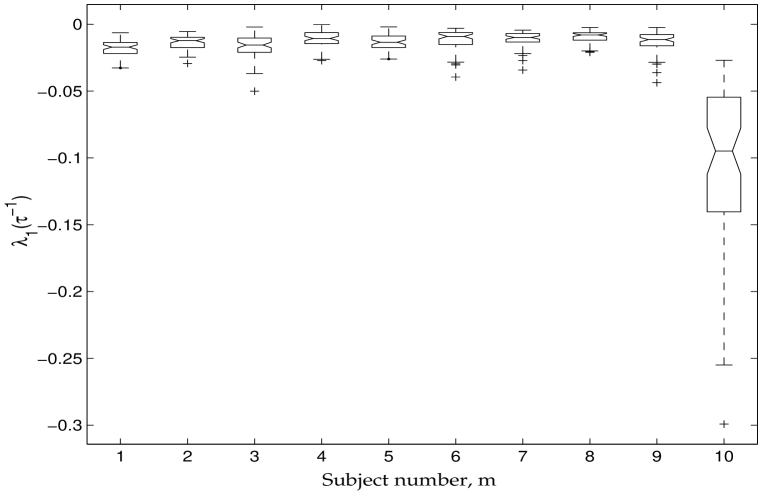
Figure 9: The mean values of the first relaxation parameter $\lambda_{1}$ for the whole group of the nine healthy subjects (n = 1, 2, 3 … 9), averaged on the total set of sensors m = 1, 2, 3,… 61 versus the patient with PSE (m = 10) for an R/ B combination of the light stimulus. One can note the drastic difference of approximately of 4,4 times for the healthy vs the patient with PSE!

From the time dependence of the initial TCF $M_{0}(t)$ and the first three MF’s of the junior order $M_{i}(t),$ i = 1, 2 and 3 it is possible to see great difference in the behavior of the time functions for the healthy and for the patient with PSE. One can observe a large-scale time correlation in the healthy subjects in the time dependence of MF’s $M_{i}(t),i=0,1,2$ and 3, whereas the similar functions demonstrate a small-scale fluctuation and a small-amplitude oscillation in case of the patient with PSE.

Figure 10: The mean values of the first relaxation parameter $\lambda_{1}$ for the group of the nine healthy subjects (m=1, 2, …9) averaged on the whole set of sensors with numbers $1\leq n\leq 61$ vs the patient with PSE (m= 10) for an R/ G combination of the light stimulus. The distinction between the healthy and the patient with PSE amounts up to 8 times!

One can note that the sensors with numbers n = 10, 5, 23, 40 and 53 are specific points in the brain core of the patient with PSE. It is interesting to observe a dynamical picture for the usual and the nonspecific points at the human cerebral cortex. To this aim, the results for the nonspecific sensor with number n = 13 are submitted in Figs. (2) - (6). Figs. (2) (for the healthy) and Figs. (5) (for the patient with PSE) present the time dependence of the first four dynamical orthogonal variables. One can detect a smooth behavior of the variables for $\ W_{i}(t)$ in the healthy and, in clear contrast, a sharp or irregular dynamics of $\ W_{i}(t)$ in the patient with PSE. Figs. (3) (for the healthy) and Figs. (6) (for the patient with PSE) show the construction of the phase space made up by separate phase points. We depict stratified phase space for the healthy person and for the patient with PSE. Figs. (4) show the nonlinear dynamics of the formation of the phase space by the phase trajectories for the healthy.

Here one can observe the pseudoperiodic orbital movement for the phase trajectory in the healthy and the quasi-strange attractors in the patient with PSE. In this context one must note the small time scales in the dynamics in the healthy and the larger time scales in nonlinear dynamics in the patient with PSE. Figs. (7) depict the time dependence of the initial TCF and the first three memory functions $M_{i}(t),$ i= 1,2 and 3 for the patient with PSE. Large scale fluctuations and oscillations are visible in the time dependence of $M_{i}(t),$ i = 0, 1, 2 and 3 in the healthy and small scale deformation are evident in the patient with the PSE.

Figs. 8 show the topographic dependence as a function of SQUID-number of the first relaxation parameters $\lambda_{1}$ for a red-blue (R/B) combinations of the light stimulus for the healthy subjects in comparison with the patient with PSE. Similar results one can see for a red-green (R/G) combinations of the light stimulus. One can observe a large difference of the numerical values of this parameter in the healthy as compared to the patient with PSE. The parameter $\lambda_{1}$ differs on average 6-7 times in the all the sensors. One can note a specially strong difference in the data between the healthy and the patient in numerical values of parameter $\lambda_{1}$ especially in the sensors with numbers n = 10, 12, 46, 51 and 56 (for an R/ B combination of the light stimulus) and n = 10, 12, 46, 51 and 53 (for an R/ G combination of light stimulus). Both combination of the light stimulus (an R/B and an R/G) yield approximately identical results for the sensor’s location.

Figs. 9 (for an R/ B combination of the light stimulus) and 10 (for an R/ G combination) demonstrate the behavior of relaxation parameter $\lambda_{1}$ for each individual of nine healthy subjects averaged on all sensor location in cerebral cortex in comparison with the patient with PSE. A remarkable difference of $\lambda_{1}$ appears in healthy subjects, this being approximately 4 - 8 times, on average 7 times for an R/ B combination in Fig. 9, and 4, 4 times for an R/G combination of the light stimulus in Fig. 10. This difference is a reliable indicator of serious destruction in functioning of the human organism with PSE. It is important that the behavior of the coefficients of $\lambda_{1}$ specifies the singularities of relaxation mechanisms in the MEG’s signals. From the physical point of view parameter $R_{1}=|\lambda_{1}|$ mimics a relaxation rate. We see the drastic distinction in relaxation rates for a healthy person as compared to the patient with PSE. This fact indicates the crucial role of the specific relaxation processes in the pathological functioning of the human cerebral cortex for the patient suffering from PSE.

One notes that the sensors with the numbers n= 10, 12, 46 and 51 locate specific points in the patient’s brain with PSE. It is necessary to mention the overall positions of the sensors. This indicates that the potential abnormality is not confined to the occipital region but distributed over the entire brain.

V Conclusions

Our discussion in this work make it evident that physiological models typically possess a great number of parameters, each with their natural range of variability and uncertainty in measurement. Relaxation and dynamic behavior of the system signals can vary widely from one chosen set of parameters to another. The presented information-theoretic memory-function analysis provides one possibility of extracting interrelations within this complicated parameter space. The study of the physical and dynamical boundaries between different types of behavior is a necessity, both for a better understanding of brain function and for the application of a diagnosing procedure and treatment of patients suffering PSE.

Control can be applied at preventing the brain from entering an undesirable, pathological state such as a seizure Parra . Here we have shown that the parameter space of MEG activity in the patient with PSE gives rise to a robust chaotic behavior. In order to study spatiotemporal cortical dynamics we need to analyze the global MEG data. In this paper we could cognize that the relaxation and dynamic singularities may account for the registration of the relevant pathological zones in the human cerebral cortex which are responsible for epilepsy.

Many natural phenomena can be described by distributions exhibiting a time scale-invariant behavior Stanley ; Worrell . The suggested approach allows the stochastic dynamics of neuromagnetic signals in human cortex to be treated in a statistical manner and to search for its characteristic statistical identifiers. From the physical point of view, the obtained results can be put to use as a possible test to identify the presence or absence of brain anomalies as they occur in a patient with PSE. The set of our quantifiers is uniquely associated with the emergence of time-scale and relaxation effects in the chaotic behavior of the neuromagnetic responses of the human brain core. The registration of the behavior of those indicators discussed here is thus of beneficial use in order to detect pathological states of separate areas (sensors 10, 5,23, 40 and 53 in our case under consideration) in the human brain of a patient with PSE.

PSE is a type of reflexive epilepsy which originates mostly in visual cortex (both striate and extra-striate) but with high possibility towards propagating to other cortical regions Binnie . Healthy brain may possess an inherent controlling (or defensive) mechanism against this propagation of cortical excitations, the breakdown of which makes the brain vulnerable to trigger epileptic seizures in patients Porciatti . However, the exact origin and dynamical nature of this putative defensive mechanism is not fully known. Earlier we showed MEG that brain responses against chromatic flickering in healthy subjects represent strong nonlinear structures whereas nonlinearity is dramatically reduced to minimal in patients.

There are other quantifiers of a different nature, such as the Lyapunov’s exponent, Kolmogorov-Sinai entropy, correlation dimension, etc., which are widely used in nonlinear dynamics and related applications, see in Ref. kantzschreiber . In the present context, we find that the employed statistical and dynamical measures are not only convenient for analysis, but are also suitable for identification of anomalous brain behavior. The search for other quantifiers, and foremost, the optimization of such measures when applied to complex discrete time dynamics presents a true challenge. This objective particularly holds true when attempts are made to identify and quantify an anomalous functioning in living systems. This study presents a first stepping stone towards understanding of nonlinear brain processes defending against hyper excitation to flickering stimulus by new analysis techniques based on non-Markov random processes.

- (1) A. M. Jade, V. K. Jayaraman, and B. D. Kulkarni, J. Phys. A: Math. Gen. 39 L483 (2006).
- (2) M. C. R. Barbosa, C. A. Linhares, and L. A. C. P. da Mota, Phys. Rev. E 74 026702 (2006).
- (3) M. Ragwitz, and H. Kantz, Phys. Rev. E, 65, 056201 (2002).
- (4) D. Marinazzo, M. Pellicoro, and S. Stramaglia, Phys. Rev. E, 73, 066216 (2006).
- (5) E. De Lauro, S. De Martino, and M. Falanga, A. Ciaramella, and R. Tagliaferri, Phys. Rev. E 72, 046712 (2005).
- (6) Y. Hirata, H. Suzuki, and K. Aihara, Phys. Rev. E 74,026202 (2006).
- (7) E. De Lauro, S. De Martino, and M. Falanga, Phys. Rev. E 74, 046712 (2005).
- (8) H. Kantz and T. Schreiber, Nonlinear Time Series Analysis (Cambridge University Press, Cambridge, UK, 1997).
- (9) F. Takens, Detecting strange attractors in turbulence, in D. A. Rand and L. - S. Young, eds., Dynamical systems and turbulence, Lecture notes in mathematics, Vol. 898, Springer, New York, 1981.
- (10) T. Sauer, J. Yorke, and M. Casdagli, J. Stat. Phys. 65, 579 (1991).
- (11) J. Stark, D. S. Broomhead, M. E. Davies, and J. Huke, Proc. 2nd World Congress of Nonlinear Analysts, Athens, Greece, 1996.
- (12) T. Sauer and J. Yorke, Int. J. Bifurcation and Chaos3, 737 (1993).
- (13) T. Schreiber, Interdisciplinary application of nonlinear time series methods, ArXiv. chao-dyn/9807001,v.1, 26 June 1998.
- (14) A. A. Markov, Proc. Phys. Math. Soc. Kazan University 15 (4), 135 (1906), in Russian.
- (15) S. Chapman and T. G. Couling, The Mathematical Theory of Nonuniform Gases (Cambridge University Press, Cambridge, 1958).
- (16) S. Albeverio, Ph. Blanchard, L. Steil, Stochastic processes and their Applications in Mathematics and Physics (Kluwer Academic Publ., 1990).
- (17) S. A. Rice, P. Gray, The Statistical Mechanics of Simple Liquids (Interscience Publ., New York, 1965).
- (18) R. Kubo, M. Toda, N. Hashitsume, N. Saito, Statistical Physics II: Nonequilibrium Statistical Mechanics (Springer Series in Solid-State Sciences 31, 279 Springer, 2003).
- (19) V. L. Ginzburg, E. Andryushin, Superconductivity (World Scientific Publ, 2004).
- (20) I. Sachs, S. Sen, J. Sexton, Elements of Statistical Mechanics (Cambridge University Press, Cambridge, 2006).
- (21) A. L. Fetter, J. D. Walecka, Quantum Theory of Many-Particle Physics (paperback) (McGraw-Hill, New York, 1971).
- (22) R. Zwanzig, Nonequilibrium Statistical Mechanics (Cambridge University Press, 2001).
- (23) D. Chandler, Introduction to Modern Statistical Mechanics (Oxford University Press, Oxford, 1987).
- (24) R. Zwanzig, Phys. Rev. 124, 983 (1961); H. Mori, Progr. Theoret. Phys. 34, 399 (1965); 33, 423 (1965).
- (25) H. Grabert, P. Hänggi, and P. Talkner, J. Stat. Phys. 22, 537 (1980); H. Grabert et al., Z. Physik B 26, 389 (1977); H. Grabert et al., Z. Physik B 29, 273 (1978); P. Hänggi and H. Thomas, Z. Physik B 26, 85 (1977); P. Hänggi and P. Talkner, Phys. Rev. Lett. 51, 2242 (1981); P. Hänggi and H. Thomas, Phys. Rep. 88, 207 (1982).
- (26) U. Balucani, M. H. Lee, V. Tognetti, Phys. Rep. 373, 409 (2003); M. H. Lee, Phys. Rev. Lett. 49, 1072 (1982); 51, 1227 (1983); J. Hong, M. H. Lee, Phys. Rev. Lett. 55, 2375 (1985); M. H. Lee, Phys. Rev. E 61, 1769, 3571 (2000); M. H. Lee, Phys. Rev. Lett. 87, 250601 (2001).
- (27) R. Kubo, Rep. Progr. Phys. 29, 255 (1966); K. Kawasaki, Ann. Phys. 61, 1 (1970); I. A. Michaels, I. Oppenheim, Physica A 81, 221 (1975); T. D. Frank, Physica D 301, 52 (2001); M. Vogt, R. Hernander, J. Chem. Phys. 123, 144109 (2005); S. Sen, Physica A. 360, 304 (2006).
- (28) M. Reed, B. Simon,The Methods of Modern Mathematical Physics,(Academic Press, New York, 1972).
- (29) C.- K. Peng, S. V. Buldyrev, S. Havlin , M. Simons, H. E. Stanley, A. L. Goldberger, Phys. Rev. E 49, 1685 (1994);. C. - K. Peng, S. Havlin, H. E. Stanley, A. L. Goldberger, Chaos 5, 82 (1995); A. L. Goldberger, L. A. N. Amaral, L. Glass, J. M. Hausdorff, P. Ch. Ivanov, R. G. Mark, J. E. Mietus, G. B. Moody, C. - K. Peng, H. E. Stanley, Circulation 101(23), e215 (2000).
- (30) A. Mokshin, R. M. Yulmetyev, P. Hanggi, Phys. Rev. Lett. 95, 200601 (2005); New J. Phys. 7, 9 (2005); R. M. Yulmetyev, F. Gafarov, P. Hanggi, R. Nigmatullin, Sh. Kayumov, Phys. Rev. E 64, 066132 (2001); R. M. Yulmetyev, P. Hanggi, F. M. Gafarov, Phys. Rev. E 65, 046107 (2002); Phys. Rev. E 62, 6178 (2000).
- (31) K. Watanabe, T. Imada, K. Nihei, S. Shimojo, Neuroreport 13, 1 (2002); J. Bhattacharya, K. Watanabe, Sh. Shimojo, Int. J. Bif. Chaos 14, 2701 (2004).
- (32) J. Parra, S. N. Kalitzin, J. Iriarte, W. Blanes, D. N. Velis, F. H. Lopes da Silva, Brain 126, 1164 (2003).
- (33) H. E. Stanley, Nature 378, 554 (1995); H. E. Stanley, Introduction to Phase Transitions and Critical Phenomena (Oxord University Press, Oxford,1971); S. Havlin, L. A. N. Amaral, Y. Ashkenazy, A. L. Goldberger, P. Ch. Ivanov, K. - C. Peng, H. E. Stanley, Physica A 274, 99 (1999); 270, 309 (1999); Z. Chen, P. Ch. Ivanov, K. Hu, and H. E. Stanley, Phys. Rev. E 65, 041107 (2002).
- (34) G. A. Worrell, S. D. Craunstoun, J. Echauz, B. Litt, NeoroReport 13, 2017 (2002).
- (35) W. A. J. Binnie, in Reflex Epilepsies and Reflex Seizures Advances in Neurology, ed. by B. Zifkin, F. Andermann, A. Beaumonir and J. Rowan (Liipincott-Raven, PA, 1998.), p. 123.
- (36) V. Porciatti, P. Bonanni, A. Fiorentini, et al., Nature Neuroscience 3, 259 (2000).