Forecasting extreme events in collective dynamics:
an analytic
signal approach to detecting discrete scale invariance
Abstract
A challenging problem in physics concerns the possibility of forecasting rare but extreme phenomena such as large earthquakes, financial market crashes, and material rupture. A promising line of research involves the early detection of precursory log-periodic oscillations to help forecast extreme events in collective phenomena where discrete scale invariance plays an important role. Here I investigate two distinct approaches towards the general problem of how to detect log-periodic oscillations in arbitrary time series without prior knowledge of the location of the moveable singularity. I first show that the problem has a definite solution in Fourier space, however the technique involved requires an unrealistically large signal to noise ratio. I then show that the quadrature signal obtained via analytic continuation onto the imaginary axis, using the Hilbert transform, necessarily retains the log-periodicities found in the original signal. This finding allows the development of a new method of detecting log-periodic oscillations that relies on calculation of the instantaneous phase of the analytic signal. I illustrate the method by applying it to the well documented stock market crash of 1987. Finally, I discuss the relevance of these findings for parametric rather than nonparametric estimation of critical times.
pacs:
05.45.Tp, 64.60.Ak, 89.65.GhI Introduction
More than a decade of pioneering research involving catastrophic phenomena as diverse as the rupture Saichev and Sornette (2005) of high pressure rocket tanks Johansen and Sornette (2000), stock market crashes Sornette and Johansen (2001) and earthquakes Saichev and Sornette (2006a) has lent growing credibility Sornette (1998, 2002) to the hypothesis that such extreme events arise due to coherent large-scale collective behaviors observed in such self-organizing systems Saichev and Sornette (2005); Sornette (1998, 2002); Johansen and Sornette (2000); Sornette and Johansen (2001); Saichev and Sornette (2006a); Bowman et al. (1998); Sornette and Sammis (1995); Huang et al. (2000a, b); Saleur et al. (1996); Saichev and Sornette (2006b, c). An exciting prospect concerns the possibility of prediction or forecasting of catastrophic events based on the observation of discrete scale invariance. This innovative approach, when applied to problems such as the prediction of earthquakes or financial crashes, questions the common assumption that the absence of characteristic scales seen in self-organizing Bak (1996); Sornette (2002) complex systems precludes the possibility of forecasting Sornette (2002). Instead, prediction becomes possible due to the appearance of smaller precursory events that in principle can help determine the critical time of the catastrophic event, which one can interpret as a finite time moveable singularity. One does not directly observe the singularity due to finite size effects. Instead we observe an ultra-large event comparable in magnitude to the system size. The best known specific signature of discrete scale invariance involves log-periodicity Sornette (1998, 2002); de Moura et al. (2000); Vallejos et al. (1998); Matsushitaa et al. (2006). Even a small improvement in the ability to detect log-periodic oscillations may thus have a relatively large impact, with potentially useful applications.
Attempts to forecast extreme events by exploiting discrete scale invariance and log-periodicity implicitly assume an underlying information-carrying property of some component in the signal studied. Indeed, in trying to forecast an event for some variable that will occur at a future time , with the information Khinchin (1957) available for at the present time , one implicitly assumes the existence of correlations in the behavior of . Such correlations imply that the knowledge of the behavior of in a certain period necessarily provides information about the behavior at other (e.g., future) times. For a continuous variable , the maximum degree of correlation arises for holomorphic or analytic , since one can then use analytic continuation to know for all future times. No new information becomes available when time elapses, because evolves deterministically. Consider the well known example of classical Hamiltonian systems. The fine grained Gibbs entropy, equivalent to the Shannon information measure, becomes a constant of the motion for such systems due to Liouville’s theorem (see ref. Zurek (1989) for a discussion of other information measures). Indeed, information can increase only if deterministic evolution becomes interrupted in some way, e.g., perhaps by some stochastic process. Such interruptions of deterministic evolution necessarily lead to breaks in analytic behavior. From such considerations, it follows as a logical consequence that the maximum possible rate of transmission of information measured in bits per unit time for a physical communication channel must equal or exceed the rate of occurrence of non-analytic points in the signal fn (1)
Detecting log-periodicity presents unique challenges. Direct parametric estimation to obtain log-periodic fits can fail due to the presence of extreme fluctuations as well as due to the problem of large degeneracy of the solutions, i.e. there exist too many good fits that approximate the best fit. Parametric methods also fail because often we do not know which underlying distribution to assume. Moreover, the large scale catastrophic events of interest may represent “outliers” that do not follow the same distribution as the smaller scale events. Hence, most of the research has tended to apply non-parametric methods.
A widely used spectroscopic method for detecting log-periodic oscillations involves changing the variable to a log-time , and then studying the power spectrum of the new series thus generated Sornette and Johansen (2001). Log-periodic oscillations will appear periodic in the log-time However, the data will no longer appear evenly sampled. Hence standard FFT-based methods do not work and instead one must obtain the spectrum via the Lomb periodogram Press et al. (1993), which can handle unevenly sampled points. In practice this method works remarkably well. Since such nonparametric methods require prior knowledge of the value of , here I investigate the general problem of how we can detect log-periodic oscillations without having prior knowledge of . Such a method would in principle allow us to “fine tune” our estimates of , and then use the nonparametric methods that rely on a priori knowledge of The methods developed here apply equally to a variety of time series, so a range of applications become possible.
In this context, one of the most dreaded collective phenomena of our times relates to the financial and economic crises that have punctuated our history since the industrial revolution. Economic events, ranging in size and diversity from the Great Depression to the ongoing bursting of the real estate bubble in the US, affect an at least order of magnitude greater number of people than earthquakes or tidal waves. Moreover, humans actively participate in the dynamics of the economy whereas we only passively watch tectonic plate movements. Indeed, financial crises have the potential to affect almost everybody (unlike, e.g., earthquakes). For such reasons, this article limits the application of the new methods developed here to the study of cooperative economic phenomena. Specifically, I have chosen to focus on the classic financial “correction” of 1987, when stock market indices dropped 20% in an amazing display of cooperative behavior (i.e., “herding”) of otherwise rational individual agents.
In Section II, I briefly review discrete scale invariance and log-periodicity. In Section III I develop techniques for detecting discrete scale invariance. In Sections IV and V I illustrate the method and then apply it to the stock market crash of 1987. Section VI concludes with a discussion and a summary.
II Complex dimensions and discrete scale invariance
The concept of dimensionality has undergone successive generalizations: from integer to fractional to negative to complex Zhou and Sornette (2006, http://arXiv.org/abs/cond-mat/0408600). The fractional and complex Saleur et al. (1996) dimensions have a relation to fractals Mandelbrot (1982); Bunde and Havlin (1991) and scale invariance symmetry, i.e., when a system’s property appears unchanged under a transformation of scale. Power laws, such as play a fundamental role in describing scale invariance. A change of scale by a factor does not alter the power law behavior: Real power law exponents usually involve continuous scale invariance. In contrast, complex exponents bear a relation to discrete scale invariance—a discrete rather than continuous symmetry that holds only for certain discrete values of the magnification . The powerful formalism that emerged from the study and exploitation of scale invariance in physical systems Stanley (1971) became known as the renormalization group (e.g., see ref. Creswick et al. (1992)). These advances have led to the application of fractal concepts and techniques to diverse systems, ranging from the study of anomalous random walks Buldyrev et al. (2001); da Luz et al. (2001) and critical points Fulco et al. (1999) to heart dynamics Viswanathan et al. (1997a) and DNA organization Viswanathan et al. (1997b); Viswanathan et al. (1998).
To model a catastrophic event that corresponds to a moveable singularity at time , we can consider an arbitrary signal in terms of the renormalization group formalism as follows:
where denotes the flow map and the critical time Johansen and Sornette (2001); Fisher (1998). The flow map acts like a “zoom,” mapping the time to a new time . We can then express as a sum of a singular part and a non-singular part as follows:
Only the singular part contributes to the ultra-large event, whereas the non-singular part only describes normal events. Close to the critical point, we can apply the linear approximation to obtain the power law solution, which satisfies
with , i.e., we essentially ignore the non-singular part. In practice this solution guarantees that continuous scale invariance shows up as straight lines on double log plots, with the slope given by , which plays the role of a fractal dimension or a scaling exponent. If we allow this dimension or exponent to become complex, , then the power law becomes , i.e., a power law modulated by oscillations with angular frequency in the logarithm of the time—hence the term log-periodic. Discrete scale invariance leads to complex exponents , with
In a number of applications, the first order representation
| (1) |
captures enough of the relevant behavior to become useful in forecasting and prediction applications Sornette and Johansen (2001). Further renormalization group symmetry considerations can lead to higher order representations useful in some cases Johansen and Sornette (2001). A different approach to extending Eq. 1 involves the inclusion of higher harmonics. However, the linear approximation leads us to expect the amplitude of the higher order log-periodic corrections to decay exponentially fast as a function of the order of the harmonics Sornette (1998). The true behavior (i.e., as opposed to the linear approximation) of the higher order harmonics leads to a slower exponential decay of the higher order harmonics. Nevertheless, the first harmonic still provides a good fit and can account for the experimental data. Having reviewed the basics of discrete scale invariance, I next address the problem of detecting it in arbitrary time series.
III Analytic behavior and discrete scale invariance
The relationship between analyticity and information flow discussed in Section I has inspired and allowed the development here of methods for detecting discrete scale invariance in arbitrary time series.
III.1 Detecting discrete scale invariance in Fourier space
How can we exploit the role of correlations to detect log-periodicity without prior knowledge of ? The power spectrum, defined as the modulus squared of the Fourier transform of the time series, allows us to measure correlations. Indeed, one could also equivalently define the power spectrum as the Fourier transform of the standard two-point autocorrelation function. As a starting point, let us consider a useful but not widely known fact about log-periodic time series and their Fourier transforms. Discrete scale invariance in a time series can sometimes also become manifest in the frequency domain.
Mathematically, log-periodicity in the time domain appears in the frequency domain because complex exponents also appear in the Fourier transform of the signal. Consider the indefinite Fourier integral
where denotes the upper incomplete Gamma function. This algebraically defined indefinite integral deals with complex quantities and represents an antiderivative with respect to the integration variable . Note the terms of the form . In practice we can evaluate this integral with lower and upper integration limits and to calculate the Fourier transform.
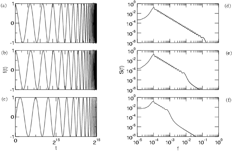
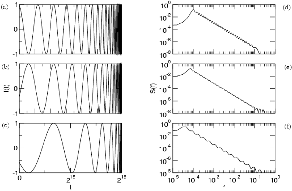
Figs. 1 and 2 show log-periodic time series and their power spectra , defined as the modulus squared of the Fourier transform of the time series. We clearly see that the log-periodicity in the time domain manifests itself as log-periodicity in the frequency domain, within a range of frequencies. Specifically, the log-periodic scaling breaks down in the spectra at low and high frequencies and the cutoff frequencies depend both on the value of as well as the temporal separation from the singularity. Except for these high and low frequency cutoffs, discrete scale invariance in the time domain manifests itself as discrete scale invariance in the frequency domain. Note that a similar relation holds for continuous scale invariance, i.e. the Fourier transform of a power law tailed function can also have a power law behavior (e.g., at low frequencies).
An increase in the critical time leads to a decrease in the upper cutoff frequency in the log-periodicity of the spectra. In principle one could exploit this relationship. Indeed, we can show in a straightforward manner that discrete scale invariance in Fourier space will break down near an upper cutoff frequency given by
| (2) |
where denotes the largest time contained in the time series. Except for too small , we can approximate
| (3) |
Hence, one could thus estimate knowing and the upper cutoff frequency in the spectra. We find that this relationship agrees fairly well for the data shown in Fig. 1. Yet, in practice I expect that this method may not work very well with real data. For realistic time series, the spectrum contains too many other features that drown out the log-periodic behavior. Perhaps one cannot systematically and reliably apply this method to detect log-periodic oscillations in realistic scenarios. Nevertheless, the concept appears to have validity on a fundamental level.
Moreover, these findings offer insight about the potential of investigating analytic behavior for detecting the crucial log-periodicities. Indeed, the basic premise of forecasting based on exploiting “hidden” analytic properties appears valid. Continuing this line of reasoning leads to a second approach. Next, I show below that the analytic signal obtained using the Hilbert transform of a time series can help to isolate the log-periodic signature in arbitrary time series. I briefly outline the method here before describing it detail below. The method involves taking the Hilbert transform of the time series to obtain the quadrature or analytic signal, consisting of the instantaneous amplitude and the instantaneous phase or argument. If the time series behaves purely log-periodically , then the phase will behave logarithmically, On the other hand, experimentally obtained data will realistically always have non-log-periodic components, so a pure log-periodic series represents an impractical idealization.
In the more realistic case of a time series with a small log-periodic component, the analytic signal phasor will rotate log-periodically in the complex plane not around the origin, but rather around some other point on the complex plane. In principle this “center” or “focus” of log-periodic rotation can itself fluctuate in time, due to the many other components that contribute to the analytic signal. Hence, in the case of a small log-periodic component in the time series, the phase of the analytic signal will not vary as . Instead the phase will have a component that oscillates log-periodically, due to the angle subtended at the origin by the analytic signal phasor tip. The log-periodicity contained in a time series need not necessarily appear in the amplitude of the analytic signal (e.g., consider how a pure log-periodic oscillation has constant amplitude). In contrast, the log-periodicity necessarily appears in the phase of the analytic signal. By studying the instantaneous phase, we may thus enhance or highlight the log-periodicity apparent in time series.
III.2 The Hilbert transform
The Hilbert transform of a function represents the convolution of the function with . Mathematically, we define the Hilbert transform as a Cauchy principal value,
to avoid the singularity at . Moreover, cancellation towards allows non-integrable functions to have well defined Hilbert transforms. The Hilbert transform also corresponds to the inverse Fourier transform of the product of the Fourier transform of with (where the latter gives the Fourier transform of ). Hence the Hilbert transform effectively maintains the Fourier amplitudes but shifts all phases by . Hence
The Hilbert transform of allows us to define an analytic signal
where and represent the instantaneous amplitude and phase of the signal. This and related properties have led Hilbert transforms to have important and diverse applications (e.g., see refs. Boashash (1992); Auyuanet et al. (2005); Zhou and Sornette (2003)).
III.3 Analytic signal of log-periodic data
For a pure log-periodic analytic signal
the “unwrapped” instantaneous phase will follow
Since in Nature we typically observe log-periodicity “decorating” a power law or else hidden in noisy data, we must consider an analytic signal of the form
with . Let . Then
and
Notice that log-periodicity need not appear in , by considering for instance, the important case , for which we obtain constant. In contrast, log-periodicity will always appear in the phase , which contains the information arising from the complex exponents associated with discrete scale invariance. The phase, calculated as an will belong to a single branch on the complex plane, but we can “unwrap” the phase to make it vary outside the conventional range to avoid abrupt discontinuities at the branch cut.
IV An illustrative example
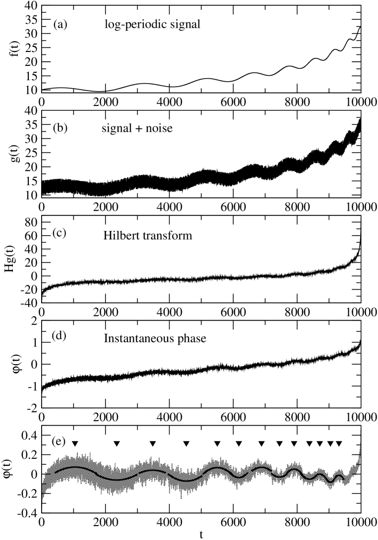
The technique developed above finds practical application to arbitrary time series. Consider, as an illustrative example, the log-periodic oscillation decorating a power law shown in Fig. 3(a). In a realistic situation, we would never observe such a clean signal. Rather, it would be embedded in noise or added to other types of signals. Fig. 3(b) shows the same log-periodic signal with noise added. Our goal involves finding the critical time from such data.
Let us thus use the signal shown in Fig. 3(b) as our test data. Applying the method described in the previous section, Fig. 3(c) shows the discrete Hilbert transform of the signal and Fig. 3(d),(e) show the instantaneous phase calculated from the analytic signal before and after detrending.
The last plot, shown in Fig. 3(e), permits an estimation of the times of the minima and maxima. I have used quadratic regression fits in the region of the extrema, due to the validity of the parabolic approximation. In principle, other methods may work equally well. Alternatively, one could estimate the times corresponding to the zeroes rather than the extrema. Yet another possibility includes direct parametric fitting of a log-periodic cosine function. I have not used this direct parametric estimation due to the reasons mentioned in Section II.
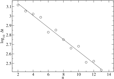
Nevertheless, knowledge of the times of the extrema permits parametric estimation of the log-periodic angular frequency Fig. 4. I have used
| (4) |
where denotes an arbitrary integer index to identify successive extrema and represent the inter-extrema intervals. The limit leads to the singularity. The regression coefficient obtained leads to a value of , compared with the known value Notice the remarkable agreement.
Once we have knowledge of and the positions of the extrema (or zeroes), it becomes straightforward to find the critical time. From Eq. (4) it follows that the inter-extrema intervals follow a geometric series defined by
| (5) |
The critical time thus satisfies
| (6) |
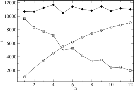
Fig. 5 shows the times , the inter-extrema intervals , and the estimated values for . We obtain an estimate for in excellent agreement with the known value.
Previous applications of the Hilbert transform to study log-periodic precursors (e.g., of financial crashes Zhou and Sornette (2003)) have assumed prior knowledge of . The log-time Zhou and Sornette (2003) behaves not log-periodically, but periodically, rendering the use of Hilbert transforms useful. In contrast, here we have assumed no prior knowledge of . Rather, such knowlegde constitutes the goal.
In summary, the method uses the following steps: (i) generation of the analytic signal from the original time series, (ii) extraction of the instantaneous phase and any necessary “unwrapping” of the phase, (iii) detrending with polynomial regression etc., (iv) testing for evidence of log-periodicity using more conventional methods. If applicable, then the final and most important step consists of estimating the location of the moveable time singularity by regression methods.
The above example illustrates step by step the application of the method to arbitrary time series. Below I apply the method to actual empirical data. Indeed, the crucial question concerns whether the method works for actual experimental data. I have chosen for this purpose the stock market crash of 1987, since it represents a well known event in which the collective social behavior of individual economic agents unleashed financial havoc and in which systematic studies have documented the role played by log-periodicities.
V The stock market crash of 1987
| Data points from Fig. 7 | Calendar dates | ||
|---|---|---|---|
| excluded | 0.076 | 9681 107 | 2/10/1987—8/8/1988 |
| excluded | 0.110 | 9419 179 | 9/6/1986—5/11/1987 |
| All points | 0.090 | 9548 86 | 24/4/1987—29/12/1987 |
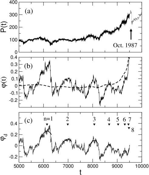
Fig. 6(a) shows data corresponding to approximately 5000 business days of the S&P500 financial index Viswanathan et al. (2003) (which has ticker symbol “SPC”). The area in grey shows the crash of October 1987, when stock markets lost some 20% of their valuation. Since the idea behind the proposed method involves forecasting the crash, I applied the method only to the data shown in black. The data in grey appears only for greater visual clarity.
Fig. 6(b) shows the instantaneous phase after detrending with polynomial regression. To emphasize the oscillations, I have further detrended the data by subtracting a uniformly weighted moving average with varying window size, using
| (7) |
where corresponds to the last point of the series. I arbitrarily have chosen 17 June 1987 as the last data point included in the test. This date corresponds to some 80 business days (i.e., several months) antecedent to the crash of October 1987.
Fig. 6(c) shows the phase after detrending with . I have estimated the positions of the maxima using using parabolic regression and have arbitrarily labelled each maxima with an index . Notice that for no sign appears of the characteristic log-periodicity. However, for the intervals between maxima become smaller, consistent with a possible log-periodicity. I have chosen to show only the maxima, because the minima appear less clear. So in what follows, note that I use a phase variation of for successive , in contrast to the a phase variation of for the inter-extrema intervals. So we must replace Eq. 5 by
| (8) |
and Eq. 6 similarly becomes
| (9) |
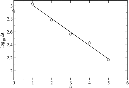
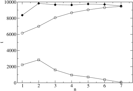
Fig. 7 shows the inter-maxima intervals . Notice the approximate exponential behavior. Using regression, we can estimate the log-periodic angular frequency . Then, we can apply Eq. 6 to estimate the crash, assuming that it should occur near the singularity. Fig. 8 shows the estimates for and Table 1 summarizes the results. All estimates contain the actual crash within the margins of error. Clearly, we must reject any estimate for that occurs within the dates studied, since we know a priori that no such event transpired.
VI Concluding remarks
Several points deserve commenting. One thought-provoking point concerns the analysis of the 1987 crash. The results reported here might bear some relation to previous findings. The very large-scale log-periodic oscillations seen in Fig. 6 are not inconsistent with similar conclusions in previous studies Sornette (2002). Such results raise a number of questions and the implications merit further study. Was the financial crisis of 1987, which few had anticipated even one month prior to the crash, really being slowly built up over large time scales spanning years? Were the individual and institutional agents really starting to behave collectively so long before the crash? What about the implication for the individual agents: is our apparently “free will” essentially irrelevant to collective dynamics?
Moreover, in the past few years, financial institutions (and some individuals) have started to use automated trading software to buy and sell financial assets (in real time Serva et al. (2006)). Each algorithmic “robo-trader” rob (15 September 2006) follows a given set of rules of arbitrary complexity, however other traders (human and robotic) do not know the specific rules and thus cannot exploit them to obtain financial arbitrage. How will the advent of large numbers of robo-traders affect the collective dynamics and what are the implications relating to the probability of financial crises?
Another noteworthy aspect concerns the the general nature of the methods developed here, whose application goes beyond financial data. One of the major difficulties in parametric estimation of log-periodic properties is due to the lack of foreknowledge of . It is not inconceivable that even small improvements in the ability to estimate can be of potential use in forecasting research. It would be interesting to apply and further study the method using other data sets. Given the recent application of physical methodologies to study music time series Jennings et al. (2004), it is even conceivable that such methods could be applied to obtain quantitative descriptions of aesthetic phenomena in the arts. In fact, wherever cooperative effects are involved, there is a real possibility that discrete scale invariance plays some role. For example, an interesting question, in this context, is whether the method is applicable to coherent noise phenomena Wilke et al. (1998); Sneppen and Newman (1997); Sornette et al. (1996). Concerning the method itself, there is room for further improvement, e.g., corrections for finite size effects of the conventionally used Hilbert transform algorithm. Similarly, one could take into consideration the role of log-periodic harmonics, which no doubt play an important role in such phenomena. Such issues are important but their relevance is secondary to the more significant question of the theoretical basis for the method. The inclusion here of further discussion about such secondary issues would detract from the central focus.
In summary, I have investigated two distinct approaches towards the general problem of how to detect log-periodic oscillations in arbitrary time series without prior knowledge of the location of critical time. The more promising method involves analytic continuation of the signal onto the imaginary axis, using the Hilbert transform. I have shown that the instantaneous phase necessarily retains the log-periodicities found in the original signal and develop a new method of detecting log-periodic oscillations. Initial results of the application of the method to the stock market crash of 1987 motivate further systematic studies to verify how much promise this approach holds for forecasting extreme events.
Acknowledgements
I thank FAPEAL, CAPES and CNPq for financial support and I. M. Gleria, F. A. B. F. de Moura, J. M. Hickmann, M. G. E. da Luz, M. L. Lyra, R. Montagne and D. Sornette for comments.
References
- Saichev and Sornette (2005) A. Saichev and D. Sornette, Phys. Rev. E 71, 016608 (2005).
- Johansen and Sornette (2000) A. Johansen and D. Sornette, Eur. Phys. J. B 18, 16 (2000).
- Sornette and Johansen (2001) D. Sornette and A. Johansen, Quantitative Finance 1, 452 (2001).
- Saichev and Sornette (2006a) A. Saichev and D. Sornette, Phys. Rev. Lett. 97, 078501 (2006a).
- Sornette (1998) D. Sornette, Physics Reports 297, 239 (1998).
- Sornette (2002) D. Sornette, P. Natl. Acad. Sci. USA 99, 2522 (2002).
- Bowman et al. (1998) D. D. Bowman, G. Ouillon, C. G. Sammis, A. Sornette, and D. Sornette, J. Geophys. Res. 103, 24359 (1998).
- Sornette and Sammis (1995) D. Sornette and C. G. Sammis, J. Phys. I 5, 607 (1995).
- Huang et al. (2000a) Y. Huang, A. Johansen, M. W. Lee, H. Saleur, and D. Sornette, J. Geophys. Res. 105, 25451 (2000a).
- Huang et al. (2000b) Y. Huang, H. Saleur, and D. Sornette, J. Geophys. Res. 105, 28111 (2000b).
- Saleur et al. (1996) H. Saleur, C. G. Sammis, and D. Sornette, J. Geophys. Res. 101, 17 (1996).
- Saichev and Sornette (2006b) A. Saichev and D. Sornette, Eur. Phys. J. B 49, 377 (2006b).
- Saichev and Sornette (2006c) A. Saichev and D. Sornette, Eur. Phys. J. B 51, 443 (2006c).
- Bak (1996) P. Bak, How Nature Works: The Science of Self-Organized Criticality (Copernicus, New York, 1996).
- de Moura et al. (2000) F. A. B. F. de Moura, U. Tirnakli, and M. L. Lyra, Phys. Rev. E 62, 6361 (2000).
- Vallejos et al. (1998) R. O. Vallejos, R. S. Mendes, L. R. da Silva, and C. Tsallis, Phys. Rev. E 58, 1346 (1998).
- Matsushitaa et al. (2006) R. Matsushitaa, S. da Silva, A. Figueiredo, and I. Gleria, Physica A 364, 331 (2006).
- Khinchin (1957) A. I. Khinchin, Mathematical Foundations of Information Theory (Dover, New York, 1957).
- Zurek (1989) W. H. Zurek, Phys. Rev. A 40, 4731 (1989).
- fn (1) As an unusual but entertaining exception, consider the anomalous pulse given by which has vanishing derivatives and peculiar properties at .
- Press et al. (1993) W. H. Press, B. P. Flannery, S. A. Teukolsky, and W. T. Vetterling, Numerical Recipes in C: The Art of Scientific Computing (Cambridge University Press, Cambridge, 1993).
- Zhou and Sornette (2006, http://arXiv.org/abs/cond-mat/0408600) W.-X. Zhou and D. Sornette (2006, http://arXiv.org/abs/cond-mat/0408600).
- Mandelbrot (1982) B. B. Mandelbrot, The Fractal Geometry of Nature (Freeman, San Fransisco, 1982).
- Bunde and Havlin (1991) A. Bunde and S. Havlin, Fractals and Disordered Systems (Springer, Berlin, 1991).
- Stanley (1971) H. E. Stanley, Introduction to Phase Transitions and Critical Phenomena (Oxford University Press, Oxford, 1971).
- Creswick et al. (1992) R. J. Creswick, H. A. Farach, and J. C. P. Poole, Introduction to Renormalization Group Methods in Physics (John Wiley & Sons, New York, 1992).
- Buldyrev et al. (2001) S. V. Buldyrev, S. Havlin, A. Y. Kazakov, M. G. E. da Luz, E. P. Raposo, H. E. Stanley, and G. M. Viswanathan, Phys. Rev. E 64, 041108 (2001).
- da Luz et al. (2001) M. da Luz, S. V. Buldyrev, S. Havlin, E. Raposo, H. E. Stanley, and G. Viswanathan, Physica A 295, 89 (2001).
- Fulco et al. (1999) U. L. Fulco, L. S. Lucena, and G. M. Viswanathan, Physica A 264, 171 (1999).
- Viswanathan et al. (1997a) G. M. Viswanathan, C.-K. Peng, H. E. Stanley, and A. L. Goldberger, Phys. Rev. E 55, 845 (1997a).
- Viswanathan et al. (1997b) G. M. Viswanathan, S. V. Buldyrev, S. Havlin, , and H. E. Stanley, Biophysical Journal 72, 866 (1997b).
- Viswanathan et al. (1998) G. M. Viswanathan, S. Buldyrev, S. Havlin, and H. Stanley, Physica A 249, 581 (1998).
- Johansen and Sornette (2001) A. Johansen and D. Sornette, Physica A 294, 465 (2001).
- Fisher (1998) M. E. Fisher, Rev. Mod. Phys. 70, 653 (1998).
- Boashash (1992) B. Boashash, Proceedings of the IEEE 80, 520 (1992).
- Auyuanet et al. (2005) A. Auyuanet, A. C. Martí, and R. Montagne, Phys. Rev. E 72, 031920 (2005).
- Zhou and Sornette (2003) W.-X. Zhou and D. Sornette, Int. J. Mod. Phys. C 14, 1107 (2003).
- Viswanathan et al. (2003) G. M. Viswanathan, U. L. Fulco, M. Lyra, and M. Serva, Physica A 329, 273 (2003).
- Serva et al. (2006) M. Serva, U. L. Fulco, I. M. Gleria, M. Lyra, F. Petroni, and G. M. Viswanathan, Physica A 363, 393 (2006).
- rob (15 September 2006) The march of the robo-traders, The Economist (15 September 2006).
- Jennings et al. (2004) H. D. Jennings, P. C. Ivanov, A. M. Martins, P. C. Silva, and G. M. Viswanathan, Physica A 336, 585 (2004).
- Wilke et al. (1998) C. Wilke, S. Altmeyer, and T. Martinetz, Physica D 120, 401 (1998).
- Sneppen and Newman (1997) K. Sneppen and M. E. J. Newman, Physica D 110, 209 (1997).
- Sornette et al. (1996) D. Sornette, L. Knopoff, Y. Kagan, and C. Vanneste, Journal Geophysical Research 101, 13883 (1996).