Mass and charge transport in micro and nano-fluidic channels

Abstract

We consider laminar flow of incompressible electrolytes in long, straight channels driven by pressure and electro-osmosis. We use a Hilbert space eigenfunction expansion to address the general problem of an arbitrary cross section and obtain general results in linear-response theory for the mass and charge transport coefficients which satisfy Onsager relations. In the limit of non-overlapping Debye layers the transport coefficients are simply expressed in terms of parameters of the electrolyte as well as the hydraulic radius ${\cal R}=2{\cal A}/{\cal P}$ with $\cal A$ and $\cal P$ being the cross-sectional area and perimeter, respectively. In particular, we consider the limits of thin non-overlapping as well as strongly overlapping Debye layers, respectively, and calculate the corrections to the hydraulic resistance due to electro-hydrodynamic interactions.

I Introduction

Laminar Hagen–Poiseuille and electro-osmotic flows are important to microfluidics and a variety of lab-on-a-chip applications Laser:04 ; Stone:04a ; Squires:05a and the rapid development of micro and nano fabrication techniques is putting even more emphasis on flow in channels with a variety of shapes depending on the fabrication technique in use. As an example the list of different geometries includes rectangular channels obtained by hot embossing in polymer wafers, semi-circular channels in isotropically etched surfaces, triangular channels in KOH-etched silicon crystals, Gaussian-shaped channels in laser-ablated polymer films, and elliptic channels in stretched soft polymer PDMS devices Geschke:04a .

In this paper we introduce our recent attempts Mortensen:05b ; Mortensen:05e in giving a general account for the mass and charge transport coefficients for an electrolyte in a micro or nanochannel of arbitrary cross sectional shape. To further motivate this work we emphasize that the flow of electrolytes in the presence of a zeta potential is a scenario of key importance to lab-on-a-chip applications involving biological liquids/samples in both microfluidic Schasfoort:1999 ; Takamura:03 ; Reichmuth:03 and nanofluidic channels Daiguji:2004 ; Stein:2004 ; Vanderheyden:2005 ; Brask:05a ; Yao:03a ; Yao:03b ; Plecis:2005 ; Schoch:2005 ; Schoch:2005a ; Jarlgaard:06 .

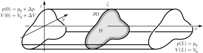
Figure 1: A translation invariant channel of arbitrary cross section $\Omega$ of area $\cal A$ containing an electrolyte driven by a pressure gradient $-\Delta p/L$ and by electro-osmosis through the potential gradient $-\Delta V/L$. The channel wall $\partial\Omega$ has the electrical potential $\zeta$, which induces a thin, charged Debye layer (dark gray) that surrounds the charge neutral bulk (light gray).

II Linear-response transport coefficients

The general steady-state flow problem is illustrated in Fig. 1 where pressure gradients and electro-osmosis (EO) are playing in concert ajdari:04a . We consider a long, straight channel of length $L$ having a constant cross section $\Omega$ of area $\cal A$ and boundary $\partial\Omega$ of length ${\cal P}$. For many purposes it is natural to introduce a single characteristic length scale

$${\cal R}=\frac{2{\cal A}}{\cal P}$$ (1)

which in the context of hydrodynamics is recognized as half the hydraulic diameter. Indeed, for a circle of radius $R$ this gives ${\cal R}=R$.

The channel contains an incompressible electrolyte, which we for simplicity assume to be binary and symmetric, i.e., containing ions of charge $+Ze$ and $-Ze$ and equal diffusivities $D$. The electrolyte has viscosity $\eta$, permittivity $\epsilon$, Debye screening length $\lambda_{D}$, and bulk conductivity $\sigma_{\mathrm{\!o}}=\epsilon D/\lambda_{D}^{2}$ and at the boundary $\partial\Omega$ it has a zeta potential $\zeta$. The laminar, steady-state transport of mass and charge is driven by a linear pressure drop $\Delta p$ and a linear voltage drop $\Delta V$. With these definitions flow will be in the positive $x$ direction. In the linear-response regime the corresponding volume flow rate $Q$ and charge current $I$ are related to the driving fields by

$$\left(\begin{array}[]{cc}Q\\ I\end{array}\right)=G\left(\begin{array}[]{cc}\Delta p\\ \Delta V\end{array}\right),\quad G=\left(\begin{array}[]{cc}G_{11}&G_{12}\\ G_{21}&G_{22}\end{array}\right),$$ (2)

where, according to Onsager relations Brunet:2004 , $G$ is a symmetric, $G_{12}=G_{21}$, two-by-two conductance matrix. In the following we introduce the characteristic conductance elements

$$G^{*}=\left(\begin{array}[]{cc}G_{\rm hyd}^{*}&G_{\rm eo}^{*}\\ G_{\rm eo}^{*}&G_{\rm mig}^{*}\end{array}\right)=\frac{\cal A}{L}\left(\begin{array}[]{cc}\frac{{\cal R}^{2}}{8\eta}&-\frac{\epsilon\zeta}{\eta}\\ -\frac{\epsilon\zeta}{\eta}&\sigma_{0}\end{array}\right),$$ (3)

which is the well-known result for a channel of circular cross section of radius $R={\cal R}\gg\lambda_{D}$.

III Summary of results

In the following we summarize our results for the transport coefficients accompanied by more heuristic arguments before we in the subsequent sections offer more detailed calculations. The upper diagonal element is the hydraulic conductance or inverse hydraulic resistance which to a good approximation is given by

$$G_{11}\approx G_{\rm hyd}^{*}.$$ (4)

While there is no intrinsic length scale influencing $G_{11}$, the other elements of $G$ depend on the Debye screening length $\lambda_{D}$. This length can be comparable to and even exceed the transverse dimensions in nano-channels Daiguji:2004 ; Stein:2004 ; Vanderheyden:2005 , in which case the off-diagonal elements may depend strongly on the actual cross-sectional geometry. However, for thin Debye layers with a vanishing overlap the matrix elements $G_{12}$, $G_{21}$, and $G_{22}$ are independent of the details of the geometry. For a free electro-osmotic flow, a constant velocity field $v_{\mathrm{eo}}=(\epsilon\zeta/\eta)\Delta V/L$ is established throughout the channel, except for in the thin Debye layer of vanishing width. Hence $Q=v_{\mathrm{eo}}{\cal A}$ and

$$G_{12}=G_{21}=G_{\rm eo}^{*},\quad\lambda_{D}\ll{\cal R}.$$ (5a)

From Ohm’s law $$I=(\sigma_{\mathrm{\!o}}{\cal A}/L)\Delta V$$ it follows that

$$G_{22}=G_{\rm mig}^{*},\quad\lambda_{D}\ll{\cal R}.$$ (5b)

For strongly overlapping Debye layers we shall see that in general

$$G_{12}=G_{21} \approx\frac{{\cal R}^{2}}{8\lambda_{D}^{2}}\>G_{\rm eo}^{*},\quad\lambda_{D}\gg{\cal R},$$ (6a)

$$G_{22} =G_{\rm mig}^{*}+{\cal O}({\cal R}^{2}/\lambda_{D}^{2}),\quad\lambda_{D}\gg{\cal R}.$$ (6b)

We emphasize that the above results are generally valid for symmetric electrolytes as well as for asymmetric electrolytes. We also note that the expressions agree fully with the corresponding limits for a circular cross section and the infinite parallel plate system, were explicit solutions exist in terms of Bessel functions Rice:65 ; Probstein:94a and cosine hyperbolic functions Probstein:94a , respectively. From the corresponding resistance matrix $R=G^{-1}$ we get the hydraulic resistance

$$R_{11}\approx\frac{1}{1-\beta}\frac{1}{G_{\rm hyd}^{*}},$$ (7a)

where $$\beta\equiv G_{12}G_{21}/(G_{11}G_{22})$$ is the Debye-layer correction factor to the hydraulic resistance. In the two limits we have

$$\beta\approx\frac{8\epsilon^{2}\zeta^{2}}{\eta\sigma_{\mathrm{\!o}}{\cal R}^{2}}\times\left\{\begin{array}[]{ccc}1&,&\displaystyle\lambda_{D}\ll{\cal R}\\ \\ \displaystyle\Big{(}\frac{{\cal R}^{2}}{8\lambda_{D}^{2}}\Big{)}^{2}&,&\displaystyle\lambda_{D}\gg{\cal R}\end{array}\right.$$ (7b)

For $\zeta$ going to zero $\beta$ vanishes and we recover the usual result for the hydraulic resistance.

IV Governing equations

For the system illustrated in Fig. 1, an external pressure gradient $\boldsymbol{\nabla}p=-(\Delta p/L){{\bf e}}_{x}$ and an external electrical field ${{\bf E}}=E{{\bf e}}_{x}=(\Delta V/L){{\bf e}}_{x}$ is applied. There is full translation invariance along the $x$ axis, from which it follows that the velocity field is of the form ${{\bf v}}({\bf{r}})=v({\bf{r}}_{\perp}){{\bf e}}_{x}$ where ${\bf{r}}_{\perp}=y{{\bf e}}_{y}+z{{\bf e}}_{z}$. For the equilibrium potential and the corresponding charge density we have $\phi_{\mathrm{eq}}({\bf{r}})=\phi_{\mathrm{eq}}({\bf{r}}_{\perp})$ and $\rho_{\mathrm{eq}}^{e}({\bf{r}})=\rho_{\mathrm{eq}}^{e}({\bf{r}}_{\perp})$, respectively. We will use the Dirac bra-ket notation Dirac:81 ; Merzbacher:70 which is mainly appreciated by researchers with a background in quantum physics, but as we shall see it allows for a very compact, and in our mind elegant, description of the present purely classical transport problem. In the following functions $f({\bf{r}}_{\perp})$ in the domain $\Omega$ are written as $\big{|}f\big{>}$ with inner products defined by the cross-section integral

$$\big{<}f\big{|}g\big{>}\equiv\int_{\Omega}d{\bf{r}}_{\perp}\,f({\bf{r}}_{\perp})g({\bf{r}}_{\perp}).$$ (8)

From the Navier–Stokes equation it follows that the velocity of the laminar flow is governed by the following force balance Batchelor:67 ; Landau:87a

$$0=\frac{\Delta p}{L}\big{|}1\big{>}+\eta\nabla_{\perp}^{2}\big{|}v\big{>}+\frac{\Delta V}{L}\big{|}\rho_{\mathrm{eq}}^{e}\big{>},$$ (9)

where $\nabla_{\perp}^{2}=\partial^{2}_{y}+\partial^{2}_{z}$ is the 2D Laplacian and $\big{|}1\big{>}$ corresponds to the unit function, i.e. $g({\bf{r}}_{\perp})=1$. The first term is the force-density from the pressure gradient, the second term is viscous force-density, and the third term is force-density transferred to the liquid from the action of the electrical field on the electrolyte ions. The equilibrium potential $\big{|}\phi_{\mathrm{eq}}\big{>}$ and the charge density $\big{|}\rho_{\mathrm{eq}}^{e}\big{>}$ are related by the Poisson equation

$$\nabla_{\perp}^{2}\big{|}\phi_{\mathrm{eq}}\big{>}=-\frac{1}{\epsilon}\big{|}\rho_{\mathrm{eq}}^{e}\big{>}.$$ (10)

The velocity $\big{|}v\big{>}$ is subject to a no-slip boundary condition on $\partial\Omega$ while the equilibrium potential $\big{|}\phi_{\mathrm{eq}}\big{>}$ equals the zeta potential $\zeta$ on $\partial\Omega$. Obviously, we also need a statistical model for the electrolyte, and in the subsequent sections we will use the Boltzmann model where the equilibrium potential $\big{|}\phi_{\mathrm{eq}}\big{>}$ is governed by the Poisson–Boltzmann equation. However, before turning to a specific model we will first derive general results which are independent of the description of the electrolyte.

We first note that because Eq. (9) is linear we can decompose the velocity as $\big{|}v\big{>}=\big{|}v_{p}\big{>}+\big{|}v_{\mathrm{eo}}\big{>}$, where $\big{|}v_{p}\big{>}$ is the Hagen–Poiseuille pressure driven velocity governed by

$$0=\frac{\Delta p}{L}\big{|}1\big{>}+\eta\nabla_{\perp}^{2}\big{|}v_{p}\big{>},$$ (11)

and $\big{|}v_{\mathrm{eo}}\big{>}$ is the electro-osmotic velocity given by

$$\big{|}v_{\mathrm{eo}}\big{>}=-\frac{\epsilon\Delta V}{\eta L}\big{(}\zeta\big{|}1\big{>}-\big{|}\phi_{\mathrm{eq}}\big{>}\big{)}.$$ (12)

The latter result is obtained by substituting Eq. (10) for $\big{|}\rho_{\mathrm{eq}}^{e}\big{>}$ in Eq. (9). The upper diagonal element in $G$ is given by $G_{11}=\big{<}1\big{|}v_{p}\big{>}/\Delta p$ which may be parameterized according to Eq. (4). The upper off-diagonal element is given by $G_{12}=\big{<}1\big{|}v_{\mathrm{eo}}\big{>}/\Delta V$ and combined with the Onsager relation we get

$$G_{12}=G_{21}=-\frac{1}{L}\frac{\epsilon}{\eta}\big{<}1\big{|}\zeta-\phi_{\mathrm{eq}}\big{>}=-\frac{{\cal A}}{L}\frac{\epsilon}{\eta}\big{(}\zeta-\bar{\phi}_{\mathrm{eq}}\big{)},$$ (13)

where we have used that $\big{<}1\big{|}1\big{>}={\cal A}$ and introduced the average potential $\bar{\phi}_{\mathrm{eq}}=\big{<}\phi_{\mathrm{eq}}\big{|}1\big{>}/\big{<}1\big{|}1\big{>}$.

There are two contributions to the lower diagonal element $G_{22}$; one from migration, $G_{22}^{\mathrm{mig}}=\big{<}1\big{|}\sigma\big{>}/L$, and one from electro-osmotic convection of charge, $G_{22}^{\mathrm{conv}}=\big{<}\rho_{\mathrm{eq}}^{e}\big{|}v_{\rm eo}\big{>}/\Delta V$, so that

$$G_{22}=G_{22}^{\mathrm{mig}}+G_{22}^{\mathrm{conv}}=\frac{1}{L}\big{<}1\big{|}\sigma\big{>}-\frac{\epsilon}{\eta L}\big{<}\rho_{\mathrm{eq}}^{e}\big{|}\zeta-\phi_{\mathrm{eq}}\big{>},$$ (14)

where the electrical conductivity $\sigma({\bf{r}}_{\perp})$ depends on the particular model for the electrolyte. For thin non-overlapping Debye layers we note that $\bar{\phi}_{\mathrm{eq}}\simeq 0$ so that Eq. (13) reduces to Eq. (5a) and, similarly since the induced charge density is low, Eq. (14) reduces to Eq. (5b). For strongly overlapping Debye layers the weak screening means that $\phi_{\mathrm{eq}}$ approaches $\zeta$ so that the off-diagonal elements $G_{12}=G_{21}$ and the $G_{22}^{\mathrm{conv}}$ part of $G_{22}$ vanish entirely. In the following we consider a particular model for the electrolyte and calculate the asymptotic suppression as a function of the Debye screening length $\lambda_{D}$.

	$\left(\kappa_{1}{\cal R}\right)^{2}$	${\cal A}_{1}^{\mathrm{eff}}/{\cal A}$	$\alpha$	$\gamma$
circle	$\gamma_{1}^{2}\simeq 5.78$a,b	$4/\gamma_{1}^{2}\simeq 0.69$a,b	$4\pi$	1c
quarter-circle	5.08d	0.65d	$29.97$d	0.93d
half-circle	5.52d	0.64d	$33.17$d	0.99d
ellipse(1:2)	6.00d	0.67d	$10\pi$c	1.05d
ellipse(1:3)	6.16d	0.62d	$40\pi/3$c	1.11d
ellipse(1:4)	6.28d	0.58d	$17\pi$c	1.14d
triangle(1:1:1)	$4\pi^{2}/9\simeq 4.39$e	$6/\pi^{2}\simeq 0.61$e	$20\sqrt{3}\>$c	$5/6\simeq 0.83$c
triangle(1:1:$\sqrt{2}$)	$\frac{5\pi^{2}}{(2+\sqrt{2})^{2}}\simeq 4.23$a	$512/9\pi^{4}\simeq 0.58$a	$38.33$d	0.82d
square(1:1)	$\pi^{2}/2\simeq 4.93$a	$64/\pi^{4}\simeq 0.66$a	$28.45$d	0.89d
rectangle(1:2)	$5\pi^{2}/9\simeq 5.48$a	$64/\pi^{4}\simeq 0.66$a	$34.98$d	0.97d
rectangle(1:3)	$5\pi^{2}/8\simeq 6.17$a	$64/\pi^{4}\simeq 0.66$a	$45.57$d	1.07d
rectangle(1:4)	$17\pi^{2}/25\simeq 6.71$a	$64/\pi^{4}\simeq 0.66$a	$56.98$d	1.14d
rectangle(1:$\infty$)	$\sim\pi^{2}\simeq 9.87$a	$64/\pi^{4}\simeq 0.66$a	$\infty$	$\sim 3/2$f
pentagon	5.20d	0.67d	$26.77$d	0.92d
hexagon	5.36d	0.68d	$26.08$d	0.94d

Table 1: Central dimensionless parameters for different geometries. ^aSee e.g. Morse:1953 for the eigenmodes and eigenspectrum. ^bHere, $\gamma_{1}\simeq 2.405$ is the first root of the zeroth Bessel function of the first kind. ^cSee e.g. Mortensen:05b and references therein. ^dData obtained by finite-element simulations comsol . ^eSee e.g. Brack:1997 for the eigenmodes and eigenspectrum. ^fSee e.g. Batchelor:67 for a solution of the Poisson equation.

V Debye–Hückel approximation

Here we will limit ourselves to the Debye–Hückel approximation while more general results beyond that approximation can be found in Ref. Mortensen:05e . In the Debye–Hückel approximation the equilibrium potential $\big{|}\phi_{\mathrm{eq}}\big{>}$ is governed by the linearized Poisson–Boltzmann equation Squires:05a

$$\nabla_{\perp}^{2}\big{|}\phi_{\mathrm{eq}}\big{>}=\frac{1}{\lambda_{D}^{2}}\big{|}\phi_{\mathrm{eq}}\big{>},$$ (15)

where $\lambda_{D}$ is the Debye screening length which for a symmetric electrolyte is given by

$$\lambda_{D}=\sqrt{\frac{\epsilon k_{B}T}{2(Ze)^{2}c_{\mathrm{o}}}}$$ (16)

with bulk concentration $c_{\mathrm{o}}$. The Debye–Hückel approximation is valid in the limit $Z\zeta e\ll k_{B}T$ where thermal energy dominates over electrostatic energy. Since we consider an open system connected to reservoirs at both ends of the channel we are able to define a bulk equilibrium concentration in the reservoirs even in the limit of strongly overlapping Debye layers inside the channel. Thus, strongly overlapping Debye layers do in this case not violate the underlying assumptions of the Poisson–Boltzmann equation.

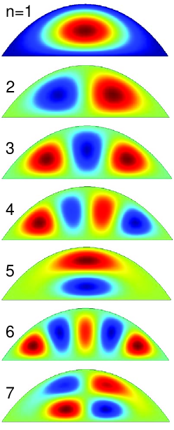
Figure 2: Examples of the first 7 eigenfunctions $\big{|}\psi_{n}\big{>}$ of Eq. (18) with the eigenvalue $\kappa_{n}^{2}$ increasing with increasing $n$. For this particular case $(\kappa_{1}{\cal R})^{2}\simeq 5.05$ and ${\cal A}_{1}/{\cal A}\simeq 0.59$ while modes with $n=2$ and $n=4$ will in this case have ${\cal A}_{n}=0$ due to the symmetry.

V.1 Hilbert space formulation

In order to solve Eqs. (9), (10), and (15) we will take advantage of the Hilbert space formulation Morse:1953 , often employed in quantum mechanics Merzbacher:70 . The Hilbert space of real functions on $\Omega$ is defined by the inner product in Eq. (8) and a complete, countable set $\big{\{}\big{|}\psi_{n}\big{>}\big{\}}$ of orthonormal basis functions, i.e.,

$$\big{<}\psi_{m}\big{|}\psi_{n}\big{>}=\delta_{nm},$$ (17)

where $\delta_{nm}$ is the Kronecker delta. As our basis functions we choose the eigenfunctions $\big{\{}\big{|}\psi_{n}\big{>}\big{\}}$ of the Helmholtz equation with a zero Dirichlet boundary condition on $\partial\Omega$,

$$-\nabla_{\perp}^{2}\big{|}\psi_{n}\big{>}=\kappa_{n}^{2}\big{|}\psi_{n}\big{>},\quad n=1,2,3,\ldots.$$ (18)

The eigenstates of Eq. (18) are well-known from a variety of different physical systems including membrane dynamics, the acoustics of drums, the single-particle eigenstates of 2D quantum dots, and quantized conductance of quantum wires. Furthermore, with an appropriate re-scaling of the Laplacian by $\cal R$ or ${\cal A}/{\cal P}$ the lowest eigenvalue has a modest dependence on the geometry Mortensen:05c ; Mortensen:05d . Fig. 2 shows as an example the 7 lowest eigenstates $\big{|}\psi_{n}\big{>}$ in a particular geometry. With this complete basis any function in the Hilbert space can be written as a linear combination of basis functions. In the following we write the fields as

$$\big{|}v\big{>} =\sum_{n=1}^{\infty}a_{n}\big{|}\psi_{n}\big{>},$$ (19a)

$$\big{|}\phi_{\mathrm{eq}}\big{>} =\zeta\big{|}1\big{>}-\sum_{n=1}^{\infty}b_{n}\big{|}\psi_{n}\big{>},$$ (19b)

$$\big{|}\rho_{\mathrm{eq}}^{e}\big{>} =\sum_{n=1}^{\infty}c_{n}\big{|}\psi_{n}\big{>}.$$ (19c)

The linear problem is now solved by straightforward bra-ket manipulations from which we identify the coefficients as

$$a_{n} =\left(\frac{\Delta p}{\eta L}\frac{1}{\kappa_{n}^{2}}-\frac{\epsilon\zeta\Delta V}{\eta L}\frac{1}{1+(\kappa_{n}\lambda_{D})^{2}}\right)\big{<}\psi_{n}\big{|}1\big{>},$$ (20a)

$$b_{n} =\zeta\frac{\big{<}\psi_{n}\big{|}1\big{>}}{1+(\kappa_{n}\lambda_{D})^{2}},$$ (20b)

$$c_{n} =-\epsilon\zeta\kappa_{n}^{2}\frac{\big{<}\psi_{n}\big{|}1\big{>}}{1+(\kappa_{n}\lambda_{D})^{2}}.$$ (20c)

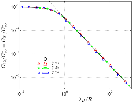
Figure 3: Rescaled off-diagonal transport coefficients versus rescaled Debye-layer thickness in the Debye–Hückel limit. The solid line is the exact result for a circle, Eq. (27), and the dashed line shows Eq. (6a). The data points are finite-element simulations for different cross sections, see inset.

V.2 Transport equations

The flow rate and the electrical current are conveniently written as

$$Q =\big{<}1\big{|}v\big{>},$$ (21a)

$$I =\big{<}\rho_{\mathrm{eq}}^{e}\big{|}v\big{>}+\sigma_{\mathrm{\!o}}E\big{<}1\big{|}1\big{>},$$ (21b)

where the second relation is the linearized Nernst–Planck equation with the first term being the convection/streaming current while the second is the ohmic current.

V.3 Transport coefficients

Substituting Eqs. (19a) and (19c) into these expressions we identify the transport coefficients as

$$G_{11} =G_{\rm hyd}^{*}\sum_{n=1}^{\infty}\frac{8}{\left(\kappa_{n}{\cal R}\right)^{2}}\frac{{\cal A}_{n}}{\cal A},$$ (22a)

$$G_{12} =G_{\rm eo}^{*}\sum_{n=1}^{\infty}\frac{1}{1+(\kappa_{n}\lambda_{D})^{2}}\frac{{\cal A}_{n}}{\cal A},$$ (22b)

$$G_{21} =G_{\rm eo}^{*}\sum_{n=1}^{\infty}\frac{1}{1+(\kappa_{n}\lambda_{D})^{2}}\frac{{\cal A}_{n}}{\cal A},$$ (22c)

$$G_{22} =G_{\rm mig}^{*}+\frac{(\epsilon\zeta)^{2}}{\eta\lambda_{D}^{2}}\frac{{\cal A}}{L}\sum_{n=1}^{\infty}\frac{(\kappa_{n}\lambda_{D})^{2}}{\big{[}1+(\kappa_{n}\lambda_{D})^{2}\big{]}^{2}}\frac{{\cal A}_{n}}{\cal A},$$ (22d)

where

$${\cal A}_{n}\equiv\frac{\big{|}\big{<}1\big{|}\psi_{n}\big{>}\big{|}^{2}}{\big{<}\psi_{n}\big{|}\psi_{n}\big{>}}=\big{|}\big{<}1\big{|}\psi_{n}\big{>}\big{|}^{2}$$ (23)

is the effective area of the eigenfunction $\big{|}\psi_{n}\big{>}$. The ratio ${\cal A}_{n}/{\cal A}$ is consequently a measure of the relative area occupied by $\big{|}\psi_{n}\big{>}$ satisfying the sum-rule $\sum_{n=1}^{\infty}{\cal A}_{n}={\cal A}$. We note that as expected $G$ obeys the Onsager relation $G_{12}=G_{21}$. Furthermore, using that

$$\frac{(\kappa_{n}\lambda_{D})^{2}}{\big{[}1+(\kappa_{n}\lambda_{D})^{2}\big{]}^{2}}=-\frac{\lambda_{D}}{2}\frac{\partial}{\partial\lambda_{D}}\frac{1}{1+(\kappa_{n}\lambda_{D})^{2}},$$ (24)

we get the following bound between the off-diagonal elements $G_{12}=G_{21}$ and the lower diagonal element $G_{22}$,

$$G_{22}=G_{\rm mig}^{*}+\frac{\epsilon\zeta}{2\lambda_{D}}\frac{\partial G_{12}}{\partial\lambda_{D}}.$$ (25)

V.4 Asymptotics and limiting cases

V.4.1 The geometrical correction factor

In analogy with Ref. Mortensen:05b we define a geometrical correction factor $\gamma\equiv G_{\rm hyd}^{*}/G_{11}$ which from Eq. (22a) becomes

$$\gamma\equiv\left(\sum_{n=1}^{\infty}\frac{8}{\left(\kappa_{n}{\cal R}\right)^{2}}\frac{{\cal A}_{n}}{\cal A}\right)^{-1}\approx\frac{\left(\kappa_{1}{\cal R}\right)^{2}}{8}\frac{\cal A}{{\cal A}_{1}}.$$ (26)

Its relation to the dimensionless parameter $\alpha$ in Ref. Mortensen:05b is $\gamma=\alpha/(2{\cal C})$ where ${\cal C}={\cal P}^{2}/{\cal A}$ is the compactness. As we shall see $\gamma$ is of the order unity and only weakly dependent on the geometry so that Eq. (4) is a good approximation for the general result in Eq. (22a).

V.4.2 Non-overlapping, thin Debye layers

For the off-diagonal elements of $G$ we use that $[1+(\kappa_{n}\lambda_{D})^{2}]^{-1}=1+{\cal O}[(\kappa_{n}\lambda_{D})^{2}]$. In Section VI we numerically justify that the smallest dimensionless eigenvalue $\kappa_{1}^{2}$ is of the order $1/{\cal R}^{2}$, so we may approximate the sum by a factor of unity, see Table 1. If we furthermore use that $\gamma\approx 1$ we arrive at Eq. (5a) for $\lambda_{D}\ll{\cal R}$. These results for the off-diagonal elements are fully equivalent to the Helmholtz–Smoluchowski result Probstein:94a . For $G_{22}$ we use that $(\kappa_{n}\lambda_{D})^{2}[1+(\kappa_{n}\lambda_{D})^{2}]^{-2}={\cal O}[(\kappa_{n}\lambda_{D})^{2}]$, thus we may neglect the second term, whereby we arrive at Eq. (5b).

V.4.3 Strongly overlapping Debye layers

In the case of $\kappa_{1}\lambda_{D}\gg 1$ we may use the result $[1+(\kappa_{n}\lambda_{D})^{2}]^{-1}=(\kappa_{n}\lambda_{D})^{-2}+{\cal O}[(\kappa_{n}\lambda_{D})^{-4}]$ which together with $\gamma\approx 1$ gives Eq. (6a) for strongly overlapping Debye layers. For $G_{22}$ we use Eq. (25) and arrive at the result in Eq. (6b).

V.4.4 The circular case

For a circular cross-section it can be shown that Probstein:94a

$$G_{12}^{\mathrm{circ}}=G_{21}^{\mathrm{circ}}=G_{\rm eo}^{*}\>\frac{I_{2}\!\big{(}{\cal R}/\lambda_{D}\big{)}}{I_{0}\!\big{(}{\cal R}/\lambda_{D}\big{)}},$$ (27)

where $I_{n}$ is the $n$th modified Bessel function of the first kind, and were we have explicitly introduced the variable ${\cal R}$ to emphasize the asymptotic dependence in Eq. (6a) for strongly overlapping Debye layers. We note that we recover the limits in Eqs. (5a) and (6a) for $\lambda_{D}\ll{\cal R}$ and $\lambda_{D}\gg{\cal R}$, respectively.

VI Numerical results

VI.1 The Helmholtz basis

Only few geometries allow analytical solutions of both the Helmholtz equation and the Poisson equation. The circle is of course among the most well-known solutions and the equilateral triangle is another example. However, in general the equations have to be solved numerically, and for this purpose we have used the commercially available finite-element software Comsol Multiphysics comsol . Fig. 2 shows the results of finite-element simulations for a particular geometry. The first eigenstate of the Helmholtz equation is in general non-degenerate and numbers for a selection of geometries are tabulated in Table 1. Note how the different numbers converge when going through the regular polygons starting from the equilateral triangle through the square, the regular pentagon, and the regular hexagon to the circle. In general, $\kappa_{1}^{2}$ is of the order $1/{\cal R}^{2}$, and for relevant high-order modes (those with a nonzero ${\cal A}_{n}$) the eigenvalue is typically much larger. Similarly, for the effective area we find that ${\cal A}_{1}/{\cal A}\leq 4/\gamma_{1}^{2}\simeq 0.69$ and consequently we have ${\cal A}_{n}/{\cal A}<1-4/\gamma_{1}^{2}\simeq 0.31$ for $n\geq 2$.

The transport coefficients in Eqs. (22a) to (22d) are thus strongly influenced by the first eigenmode which may be used for approximations and estimates of the transport coefficients. As an example the column for $\gamma$ is well approximated by only including the first eigenvalue in the summation in Eq. (26). In fact, the approximation $\gamma\approx 1$ is indeed reasonable.

VI.2 Transport coefficients

Our analytical results predict that when going to either of the limits of thin non-overlapping or strongly overlapping Debye layers, the transport coefficients to a good approximation only depend on the channel geometry through the hydraulic radius ${\cal R}$. Therefore, when plotted against the rescaled Debye length $\lambda_{D}/{\cal R}$, all our results should collapse on the same asymptotes in the two limits.

In Fig. 3 we show the results for the off-diagonal coefficients obtained from finite-element simulations in the Debye–Hückel limit for three different channel cross sections, namely two parabola shaped channels of aspect ratio 1:1 and 1:5, respectively, and a rectangular channel of aspect ratio 1:5. In all cases we find excellent agreement between the numerics and the asymptotic expressions. For the comparison we have also included exact results, Eq. (27), for the circular cross section as well as results based on only the first eigenvalue in Eq. (22b). Even though Eq. (27) is derived for a circular geometry we find that it also accounts remarkably well for even highly non-circular geometries in the intermediate regime of weakly overlapping Debye layers.

VII Conclusion

We have analyzed the flow of incompressible electrolytes in long, straight channels driven by pressure and electro-osmosis. By using a powerful Hilbert space eigenfunction expansion we have been able to address the general problem of an arbitrary cross section and obtained general results for the hydraulic and electrical transport coefficients. Results for strongly overlapping and thin, non-overlapping Debye layers are particular simple, and from these analytical results we have calculated the corrections to the hydraulic resistance due to electro-hydrodynamic interactions. These analytical results reveal that the geometry dependence only appears through the hydraulic radius ${\cal R}$ and the correction factor $\gamma$, as the expressions only depend on the rescaled Debye length $\lambda_{D}/{\cal R}$ and $\gamma\approx 1$. Our numerical analysis based on finite-element simulations indicates that these conclusions are generally valid also for intermediate values of $\lambda_{D}$. The present results constitute an important step toward circuit analysis Brask:03a ; ajdari:04a of complicated micro and nanofluidic networks incorporating complicated cross-sectional channel geometries.

References

- (1) D. J. Laser and J. G. Santiago, “A review of micropumps,” J. Micromech. Microeng., vol. 14, no. 6, pp. R35 – R64, 2004.
- (2) H. A. Stone, A. D. Stroock, and A. Ajdari, “Engineering flows in small devices: Microfluidics toward a lab-on-a-chip,” Annu. Rev. Fluid Mech., vol. 36, pp. 381 – 411, 2004.
- (3) T. M. Squires and S. R. Quake, “Microfluidics: Fluid physics at the nanoliter scale,” Rev. Mod. Phys., vol. 77, pp. 977 – 1026, 2005.
- (4) O. Geschke, H. Klank, and P. Telleman, Eds., Microsystem Engineering of Lab-on-a-Chip Devices. Weinheim: Wiley-VCH Verlag, 2004.
- (5) N. A. Mortensen, F. Okkels, and H. Bruus, “Reexamination of Hagen–Poiseuille flow: Shape dependence of the hydraulic resistance in microchannels,” Phys. Rev. E, vol. 71, p. 057301, 2005.
- (6) N. A. Mortensen, L. H. Olesen, and H. Bruus, “Transport coefficients for electrolytes in arbitrarily shaped nano and micro-fluidic channels,” New J. Phys., vol. 8, p. 37, 2006.
- (7) R. B. M. Schasfoort, S. Schlautmann, L. Hendrikse, and A. van den Berg, “Field-effect flow control for microfabricated fluidic networks,” Science, vol. 286, no. 5441, pp. 942 – 945, 1999.
- (8) Y. Takamura, H. Onoda, H. Inokuchi, S. Adachi, A. Oki, and Y. Horiike, “Low-voltage electroosmosis pump for stand-alone microfluidics devices,” Electrophoresis, vol. 24, no. 1-2, pp. 185 – 192, 2003.
- (9) D. S. Reichmuth, G. S. Chirica, and B. J. Kirby, “Increasing the performance of high-pressure, high-efficiency electrokinetic micropumps using zwitterionic solute additives,” Sens. Actuator B-Chem., vol. 92, no. 1-2, pp. 37 – 43, 2003.
- (10) H. Daiguji, P. D. Yang, A. J. Szeri, and A. Majumdar, “Electrochemomechanical energy conversion in nanofluidic channels,” Nano Lett., vol. 4, no. 12, pp. 2315 – 2321, 2004.
- (11) D. Stein, M. Kruithof, and C. Dekker, “Surface-charge-governed ion transport in nanofluidic channels,” Phys. Rev. Lett., vol. 93, no. 3, p. 035901, 2004.
- (12) F. H. J. van der Heyden, D. Stein, and C. Dekker, “Streaming currents in a single nanofluidic channel,” Phys. Rev. Lett., vol. 95, no. 11, p. 116104, 2005.
- (13) A. Brask, J. P. Kutter, and H. Bruus, “Long-term stable electroosmotic pump with ion exchange membranes,” Lab Chip, vol. 5, no. 7, pp. 730 – 738, 2005.
- (14) S. H. Yao and J. G. Santiago, “Porous glass electroosmotic pumps: theory,” J. Colloid Interface Sci., vol. 268, no. 1, pp. 133 – 142, 2003.
- (15) S. H. Yao, D. E. Hertzog, S. L. Zeng, J. C. Mikkelsen, and J. G. Santiago, “Porous glass electroosmotic pumps: design and experiments,” J. Colloid Interface Sci., vol. 268, no. 1, pp. 143 – 153, 2003.
- (16) A. Plecis, R. B. Schoch, and P. Renaud, “Ionic transport phenomena in nanofluidics: Experimental and theoretical study of the exclusion-enrichment effect on a chip,” Nano Lett., vol. 5, no. 6, pp. 1147 – 1155, 2005.
- (17) R. B. Schoch, H. van Lintel, and P. Renaud, “Effect of the surface charge on ion transport through nanoslits,” Phys. Fluids, vol. 17, no. 10, p. 100604, 2005.
- (18) R. B. Schoch and P. Renaud, “Ion transport through nanoslits dominated by the effective surface charge,” Appl. Phys. Lett., vol. 86, no. 25, p. 253111, 2005.
- (19) S. E. Jarlgaard, M. B. L. Mikkelsen, P. Skafte-Pedersen, H. Bruus, and A. Kristensen, “Capillary filling speed in silicon dioxide nano-channels,” in Proc. NSTI-Nanotech 2006, vol. 2, 2006, pp. 521 – 523.
- (20) A. Ajdari, “Steady flows in networks of microfluidic channels: building on the analogy with electrical circuits,” C. R. Physique, vol. 5, pp. 539 – 546, 2004.
- (21) E. Brunet and A. Ajdari, “Generalized onsager relations for electrokinetic effects in anisotropic and heterogeneous geometries,” Phys. Rev. E, vol. 69, no. 1, p. 016306, 2004.
- (22) C. L. Rice and R. Whitehead, “Electrokinetic flow in a narrow cylindrical capillary,” J. Phys. Chem., vol. 69, no. 11, pp. 4017 – 4024, 1965.
- (23) R. F. Probstein, PhysicoChemical Hydrodynamics, an introduction. New-York: John Wiley and Sons, 1994.
- (24) P. A. M. Dirac, The Principles of Quantum Mechanics, 4th ed. Oxford: Oxford University Press, 1981.
- (25) E. Merzbacher, Quantum Mechanics. New York: Wiley & Sons, 1970.
- (26) G. K. Batchelor, An Introduction to Fluid Dynamics. Cambridge: Cambridge University Press, 1967.
- (27) L. D. Landau and E. M. Lifshitz, Fluid Mechanics, 2nd ed., ser. Landau and Lifshitz, Course of Theoretical Physics. Oxford: Butterworth–Heinemann, 1987, vol. 6.
- (28) P. M. Morse and H. Feshbach, Methods of Theoretical Physics. New York: McGraw–Hill, 1953.
- (29) Comsol support and Femlab documentation, www.comsol.com.
- (30) M. Brack and R. K. Bhaduri, Semiclassical Physics. New York: Addison Wesley, 1997.
- (31) N. A. Mortensen, F. Okkels, and H. Bruus, “Universality in edge-source diffusion dynamics,” Phys. Rev. E, vol. 73, p. 012101, 2006.
- (32) N. A. Mortensen and H. Bruus, “Universal dynamics in the onset of a hagen-poiseuille flow,” Phys. Rev. E, vol. 74, p. 017301, 2006.
- (33) A. Brask, G. Goranović, and H. Bruus, “Theoretical analysis of the low-voltage cascade electroosmotic pump,” Sens. Actuator B-Chem., vol. 92, pp. 127–132, 2003.