What is the Time Scale of Random Sequential Adsorption?

Abstract

A simple multiscale approach to the diffusion-driven adsorption from a solution to a solid surface is presented. The model combines two important features of the adsorption process: (i) the kinetics of the chemical reaction between adsorbing molecules and the surface; and (ii) geometrical constraints on the surface made by molecules which are already adsorbed. The process (i) is modelled in a diffusion-driven context, i.e. the conditional probability of adsorbing a molecule provided that the molecule hits the surface is related to the macroscopic surface reaction rate. The geometrical constraint (ii) is modelled using random sequential adsorption (RSA), which is the sequential addition of molecules at random positions on a surface; one attempt to attach a molecule is made per one RSA simulation time step. By coupling RSA with the diffusion of molecules in the solution above the surface the RSA simulation time step is related to the real physical time. The method is illustrated on a model of chemisorption of reactive polymers to a virus surface.

Random sequential adsorption (RSA) is a classical model of irreversible adsorption (e.g. chemisorption) Evans (1993). Given a sequence of times $t_{k}$, $k=1,2,3,\dots$, an attempt is made to attach one object (e.g. a molecule) to the surface at each time point $t=t_{k}$. If the attempt is successful (i.e. if there is enough space on the surface to place the molecule), the object is irreversibly adsorbed. It cannot further move or leave the structure and it covers part of the surface, preventing other objects from adsorbing in its neighbourhood (e.g. by steric shielding in the molecular context).

In the simplest form, RSA processes are formulated as attempting to place one object per RSA time step, expressing the simulation time in units equal to the number of RSA time steps $k$ rather than in real physical time $t_{k}$. Such an approach is useful to compute the maximal (jamming) coverage of the surface. To apply RSA models to dynamical problems, it is necessary to relate the time of the RSA simulation $k$ and the real time $t_{k}$. This is a goal of this paper. We consider that the adsorbing objects are molecules which can covalently attach to the binding sites on the surface. We couple the RSA model with processes in the solution above the surface to study the irreversible adsorption of molecules in real time. The time $(t_{k}-t_{k-1})$ between the subsequent attempts to place a molecule is in general a non-constant function of $k$ which depends on the kinetics of the chemical reaction between the adsorbing molecules and the surface, and on the stochastic reaction-diffusion processes in the solution above the surface. We illustrate our method with an example of the chemisorption of reactive polymers to a virus surface Erban et al. ; Erban and Chapman (a). Finally, we show that the stochastic simulation in the solution can be substituted by a suitable deterministic partial differential equation which decreases the computational intensity of the algorithm. We show that it is possible to get the values of $t_{k}$ without doing extensive additional stochastic simulations.

We consider a three-dimensional cuboid domain $L_{x}\times L_{x}\times L_{z}$ in which molecules diffuse (see Fig. 1). The side $z=0$ of area $L_{x}\times L_{x}$ is assumed to be adsorbing, i.e. containing binding sites to which molecules can covalently attach. Our goal is to couple RSA on the side $z=0$ with stochastic reaction-diffusion processes in the solution above the adsorbing surface. Since those molecules which are far from the surface will have little influence on the adsorbtion process, it is a waste of resources

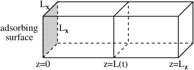
Figure 1: Three-dimensional cuboid domain.

to compute their trajectories. We will therefore carefully truncate our computational domain to that which is effectively influenced by the reactive boundary at $z=0$, which we denote by $z<L(t)$. Note that $L(t)$ is not fixed but a function of time—the formula for it will be derived later. Suppose that there are $N(t)$ diffusing molecules in the cuboid domain $L_{x}\times L_{x}\times L(t)$. Let us denote the $z$-coordinate of the $i$-th molecule by $z_{i}(t)$, treating molecules as points in the solution in what follows. Choosing a time step $\Delta t$, we compute $z_{i}(t+\Delta t)$ from $z_{i}(t),$ $i=1,\dots,N(t),$ by

$$z_{i}(t+\Delta t)=z_{i}(t)+\sqrt{2D_{i}\,\Delta t}\;\xi_{i},$$ (1)

where $\xi_{i}$ is a normally distributed random variable with zero mean and unit variance and $D_{i}$ is the diffusion constant of the $i$-th molecule. In principle, we should model the behaviour of molecules as three dimensional random walks in the cuboid domain $L_{x}\times L_{x}\times L(t)$, i.e. there should be equations analogous to (1) for the $x$ and $y$ coordinates too. However, we can often assume that $L(t)\gg L_{x}$ in applications. Choosing the time step $\Delta t$ large enough that a molecule travels over distances comparable to $L_{x}$ during one time step, we can assume that the molecules are effectively well-mixed in the $x$ and $y$ directions on this time scale. Consequently, the $x$ and $y$ coordinates of molecules do not have to be simulated. If the original adsorbing surface is large, one often models by RSA only a representative part of it, i.e. a square $L_{x}\times L_{x}$ which contains a relatively large number of binding sites, but still satisfies $L_{x}\ll L(t)$. The diffusion of molecules (1) is coupled with other processes in the solution and on the surface as follows.

Chemical reactions in the solution: Our illustrative example is the polymer coating of viruses Erban et al. ; Erban and Chapman (a). In this case, the polymer molecules have reactive groups which can covalently bind to the surface. The reactive groups also hydrolyse in solution. Assuming that there is one reactive group per polymer molecule (such a polymer is called semitelechelic), we have effectively one chemical reaction in the solution - a removal of the reactive polymers from the solution with rate $\lambda$ Šubr et al. (2006). Assuming that $\lambda\Delta t\ll 1$, the stochastic modelling of the process in the solution is straightforward. At each time step, the $i$-th molecule moves according to (1). We then generate a random number $r_{i}$ uniformly distributed on the interval $[0,1]$. If $r_{i}<\lambda\Delta t$, we remove the molecule from the system. More complicated reaction mechanisms in the solution can be treated using stochastic simulation algorithms which have been proposed for reaction-diffusion processes in the literature Andrews and Bray (2004); Hattne et al. (2005); Isaacson and Peskin (2006). In our case, we treat diffusion using the discretized version of Smoluchowski equation (1). Consequently, we can follow Andrews and Bray Andrews and Bray (2004) to introduce higher-order reactions to the system.

Adsorption to the surface: The surface $L_{x}\times L_{x}$ at $z=0$ is assumed to be adsorbing. We use a simple version of the RSA model from Erban and Chapman (a) which postulates that the binding sites on the surface lie on a rectangular lattice. Binding a polymer to a lattice site prevents the binding of another polymer to the neighbouring lattice sites through steric shielding, i.e. we consider RSA with the nearest neighbour exclusion as a toy model of adsorption Evans (1993). Such a RSA model can be simulated on its own as shown in Erban and Chapman (a). In this paper, we simulate it together with the $z$-variables of molecules in the solution (1) to get the RSA evolution in real physical time. Whenever a molecule hits the boundary $z=0$, it is adsorbed with some probability, and reflected otherwise. This partially adsorbing boundary condition is implemented in the RSA context as follows:

(a) If $z_{i}(t+\Delta t)$ computed by (1) is negative then, with probability $P\sqrt{\Delta t}$, we attempt one step of the RSA algorithm with the $i$-th molecule. If the $i$-th molecule is adsorbed, we remove it from the solution. Otherwise, we put $z_{i}(t+\Delta t)=-z_{i}(t)-\sqrt{2D_{i}\,\Delta t}\;\xi_{i}$.

(b) If $z_{i}(t+\Delta t)$ computed by (1) is positive then, with probability $\exp[-x_{i}(t)x_{i}(t+\Delta t)/(D\Delta t)]P\sqrt{\Delta t}$, we attempt one step of the RSA algorithm with the $i$-th molecule. If the $i$-th molecule is adsorbed, we remove it from the solution.

Here, $P$ is a positive constant which can be related to the rate constant of the chemical reaction between the binding sites on the virus surface and the reactive groups on the polymer Erban and Chapman (b). This relation depends on the stochastic model of diffusion and for equation (1) is given later – see formula (6). Conditions (a)–(b) state that only the fraction $P\sqrt{\Delta t}$ of molecules which hit the boundary have a chance to create a chemical bond (provided that there is no steric shielding). Obviously, if $z_{i}(t+\Delta t)$ computed by (1) is negative, a molecule has hit the boundary. This case is incorporated in (a). However, Andrews and Bray Andrews and Bray (2004) argue that there is a chance that a molecule hit the boundary during the finite time step $\Delta t$ even if $z_{i}(t+\Delta t)$ computed by (1) is positive; that is, during the time interval $[t,t+\Delta t]$ the molecule might have crossed to $z_{i}$ negative and then crossed back to $z_{i}$ positive again. They found that the probability that the molecule hit the boundary $z=0$ at least once during the time step $\Delta t$ is $\exp[-z_{i}(t)z_{i}(t+\Delta t)/(D\Delta t)]$ for $z_{i}(t)\geq 0$, $z_{i}(t+\Delta t)\geq 0$. This formula is used in (b).

​​​​​​

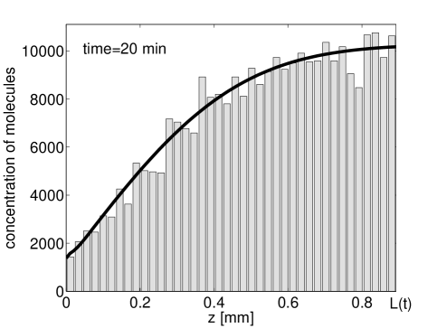
Figure 2: Concentration of polymer molecules in the solution above the adsorbing surface $z=0$ at times 20 and 80 minutes.

Numerical results: It is important to note that the boundary conditions (a)–(b) can be used for any RSA algorithm and for any set of reactions in the solution. To apply it to the virus coating problem, we have to specify some details of the model. First of all, it can be estimated that the average distance between the binding sites is about 1 nm Erban et al. . We choose $L_{x}=100$ nm. Therefore, there are about $10,000$ binding sites on the adsorbing side $z=0$. We use RSA on a $100\times 100$ lattice with the nearest neighbour exclusion, which is a special case of the model from Erban and Chapman (a). We consider a monodisperse solution of semitelechelic 50 kDa polymers, i.e. $D_{i}\equiv D$ where $D=5\times 10^{-5}\;\mbox{mm}^{2}\;\mbox{s}^{-1}$ Prokopová-Kubinová et al. (2001). The rate of hydrolysis of the reactive groups on polymers can be estimated from data in Šubr et al. (2006) as $\lambda=1.3\times 10^{-4}\,\mbox{s}^{-1}.$ We choose $P=1\;\mbox{s}^{-1/2}$. Since we simulate the behaviour of polymer molecules in solution only along the $z$-direction, we express the concentration of polymer $c(z,t)$ in numbers of polymer molecules per volume $L_{x}\times L_{x}\times[1\;\mbox{mm}]$ where $L_{x}=10^{-4}$ mm is fixed. A typical experiment starts with a uniform concentration of reactive polymers. Considering that the initial concentration of 50 kDa polymer is 0.1 g/l, we obtain the initial condition $c_{0}=1.2\times 10^{4}$ molecules per mm of the height above the surface (let us note that the units of the “one-dimensional” concentration $c(z,t)$ are molecules/mm because $L_{x}$ is considered fixed). Next, we have to specify $L(t)$ (see Fig. 1), i.e. we want to find the region of the space which is effectively influenced by the boundary condition at $z=0$. To that end, we note that the concentration $c(z,t)$ satisfies the partial differential equation

$$\frac{\partial c}{\partial t}=D\frac{\partial^{2}c}{\partial z^{2}}-\lambda c.$$ (2)

Now any partially reacting boundary will have less impact on the spatial profile of $c(z,t)$ than perfect adsorption at $z=0$. Thus we may find an upper bound for the region of influence of the boundary by solving (2) subject to

$$c(0,t)=0,\qquad\lim_{z\to\infty}c(z,t)=c_{0}\exp[-\lambda t],$$ (3)

for $t\in[0,\infty)$, and the initial condition $c(z,0)=c_{0},$ for $z\in[0,\infty)$. The solution of (2)–(3) is

$$c(z,t)=c_{0}\exp[-\lambda t]\mathop{\mbox{erf}}\left(\frac{z}{2\sqrt{Dt}}\right)$$ (4)

where $\mathop{\mbox{erf}}(\cdot)$ denotes the error function. Defining $\omega=\mbox{erf}^{-1}(0.99)\doteq 1.821$ we set

$$L(t)\equiv 2\omega\sqrt{Dt}.$$ (5)

Then $c(L(t),t)=0.99\,c_{0}\exp[-\lambda t]$, so that the concentration of the reactive polymer at point $z=L(t)$ at time $t$ is equal to 99 % of the polymer concentration at points which are “infinitely far” from the adsorbing boundary. In particular, we can assume that the adsorbing boundary effectively influences the polymer concentration only at heights $z\in[0,L(t)]$ above the boundary and we can approximate $c(z,t)\sim c_{0}\exp[-\lambda t]$ for $z>L(t).$ Formula (5) specifies the computational domain as $L_{x}\times L_{x}\times L(t)$ at each time (see Fig. 1).

The results of the stochastic simulation of the solution above the surface are shown in Fig. 2 as grey histograms. To simulate the behaviour of $N(t)$ reactive polymers, we consider only their $z$-positions. We use $\Delta t=10^{-2}$ s and we update the $z$-positions of molecules during one time step according to (1). At each time step, we also generate a uniformly distributed random number $r_{i}$ and we remove the $i$-th molecule from the system if $r_{i}<\lambda\,\Delta t$. We work in the one-dimensional domain $[0,L(t)]$ where $L(t)$ is given by (5). The RSA boundary condition at $z=0$ is implemented using (a)–(b) described above. The right boundary increases during one time step by $\Delta L(t)=L(t+\Delta t)-L(t)$. During each time step, we have to put on average $m(t)=c_{0}\exp[-\lambda t]\Delta L(t)$ molecules into the interval $[L(t),L(t+\Delta t)]$. This is done as follows. We put $\lfloor m(t)\rfloor$ molecules at random positions in the interval $[L(t),L(t+\Delta t)]$, where $\lfloor\cdot\rfloor$ denotes the integer part. Moreover, we generate random number $r_{\Delta t}$ uniformly distributed in $[0,1]$ and we add one molecule at a random position in the interval $[L(t),L(t+\Delta t)]$ if $r_{\Delta t}<m(t)-\lfloor m(t)\rfloor.$ This will ensure that we put on average $m(t)$ molecules to the interval $[L(t),L(t+\Delta t)]$ during one time step.

Introducing the moving boundary decreases the computational intensity of the model. Initially we simulate a relatively small region with a high concentration of reactive polymers. The simulated region increases with time but the concentration of reactive molecules decreases with rate $\lambda$. Using (4), it can be computed that the maximal number of simulated polymers in solution is achieved at time $t_{m}=(2\lambda)^{-1}\doteq 64$ min (and is about $8\times 10^{3}$ molecules for our parameter values).

The number of polymers adsorbed to the RSA surface at $z=0$ as a function of real physical time is shown in Fig. 3. Since the polymer solution is assumed to be monodisperse, we can run the RSA algorithm first and record the times $k_{1},$ $k_{2}$, $k_{3}$, …(expressed in numbers of the RSA time steps) of successful attempts to place the polymer on the RSA lattice. Then the stochastic simulation of the reaction-diffusion processes in the solution can use $k_{1},$ $k_{2}$, $k_{3}$, …as its input. We will shortly consider another approach to the problem, replacing the stochastic simulation of the solution by the continuum limit (2) with a suitable Robin boundary condition. To enable a direct comparison of the two approaches, we use the same sequence $k_{1},$ $k_{2}$, $k_{3}$, …in ten realizations of the full stochastic model of adsorption; the results are shown as grey solid lines in Fig. 3.

  

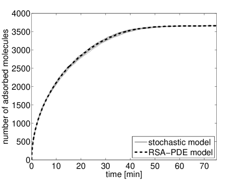
Figure 3: Number of polymer molecules adsorbed to the RSA lattice as a function of the real physical time.

RSA-PDE approach: Moving the right boundary $L(t)$ is one way to decrease the computational intensity of the problem. Another possibility is to use the deterministic equation (2) together with a Robin boundary condition

$$\frac{\partial c}{\partial z}(0,t)=\alpha_{RSA}(t)\frac{2P}{\sqrt{D\pi}}\,\,c(0,t)$$ (6)

at the adsorbing boundary $z=0$. Here, the fraction $2P/\sqrt{D\pi}$ corresponds to the rate of the chemical reaction between the adsorbing boundary and the diffusing molecules in the solution – see Erban and Chapman (b) for the derivation of this formula and further discussion. Factor $\alpha_{RSA}(t)\in\{0,1\}$ provides the coupling between the RSA model and (2). To find the value of $\alpha_{RSA}(t)$, we estimate the number of attempts to place the polymer on the RSA lattice by

$$\kappa(t)=\left\lfloor\int_{0}^{t}\frac{2P\sqrt{D}}{\sqrt{\pi}}c(0,t)\mbox{d}t\right\rfloor$$

where $\lfloor\cdot\rfloor$ denotes the integer part Erban and Chapman (b). We start with $\alpha_{RSA}(t)=1$ and we solve (2) and (6) numerically. Whenever $\kappa(t)$ increases by 1, we attempt one step of the RSA. If the attempt is successful, we put $\alpha_{RSA}(t)=1$. If the attempt to place the molecule is not successful, we put $\alpha_{RSA}(t)=0$. Thus $\alpha_{RSA}(t)$ has only two values, 0 and 1, and changes at computed time points depending on the output of the RSA simulation. We call this procedure the RSA-PDE approach. It also leads to the sequence of real physical times $t_{k_{1}}$, $t_{k_{2}}$, $t_{k_{3}}$ $\dots$, of successful attempts to place the polymer on the RSA lattice. The numerical solution of equation (2) with the Robin boundary condition (6) at $z=0$ is presented in Fig. 2 as the solid line for comparison. We also plot the number of adsorbed polymers as a function of the real time as the dashed line in Fig. 3. To enable the direct comparison, we run the RSA algorithm first and we record the times of successful attempts to place the polymer on the lattice. We obtain the sequence $k_{1},$ $k_{2}$, $k_{3}$, …of times expressed in number of RSA time steps. This sequence is used in both the stochastic model (10 realizations plotted in Fig. 3 as grey solid lines) and the RSA-PDE approach (dashed line in Fig. 3). The comparison of the results obtained by the full stochastic model and by the RSA-PDE model is excellent.

Conclusion: We have presented a method to perform RSA simulation in real physical time. The key part of the method is the boundary condition (a)–(b) which can be coupled with any reaction-diffusion model in the solution and any RSA algorithm. We illustrated this fact on a simple model of the polymer coating of viruses. Moreover, we showed that the RSA algorithm can be coupled with (2) using the Robin boundary condition (6) to get comparable results. The Robin boundary condition (6) is also not restricted to our illustrative example. It can be used for the coupling of any RSA model with the PDE model of the reaction-diffusion processes in the solution above the adsorbing surface.

Acknowledgments: This work was supported by the Biotechnology and Biological Sciences Research Council.

References

- Evans (1993) J. Evans, Reviews of Modern Physics 65, 1281 (1993).
- (2) R. Erban, S. J. Chapman, K. Fisher, I. Kevrekidis, and L. Seymour, 22 pages, to appear in Mathematical Models and Methods in Applied Sciences (M3AS), available as arxiv.org/physics/0602001, 2006.
- Erban and Chapman (a) R. Erban and S. J. Chapman, to appear in Journal of Statistical Physics, available as arxiv.org/physics/0609029, 2006.
- Šubr et al. (2006) V. Šubr, Č. Koňák, R. Laga, and K. Ulbrich, Biomacromolecules 7, 122 (2006).
- Andrews and Bray (2004) S. Andrews and D. Bray, Physical Biology 1, 137 (2004).
- Hattne et al. (2005) J. Hattne, D. Fagne, and J. Elf, Bioinformatics 21, 2923 (2005).
- Isaacson and Peskin (2006) S. Isaacson and C. Peskin, SIAM Journal on Scientific Computing 28, 47 (2006).
- Erban and Chapman (b) R. Erban and S. J. Chapman, 24 pages, submitted to Physical Biology, available as arxiv.org/physics/0611251, 2006.
- Prokopová-Kubinová et al. (2001) Š. Prokopová-Kubinová, L. Vargová, L. Tao, K. Ulbrich, V. Šubr, E. Syková, and C. Nicholson, Biophysical Journal 80, 542 (2001).