Realistic boundary conditions for stochastic simulations of reaction-diffusion processes

Abstract

Many cellular and subcellular biological processes can be described in terms of diffusing and chemically reacting species (e.g. enzymes). Such reaction-diffusion processes can be mathematically modelled using either deterministic partial-differential equations or stochastic simulation algorithms. The latter provide a more detailed and precise picture, and several stochastic simulation algorithms have been proposed in recent years. Such models typically give the same description of the reaction-diffusion processes far from the boundary of the simulated domain, but the behaviour close to a reactive boundary (e.g. a membrane with receptors) is unfortunately model-dependent. In this paper, we study four different approaches to stochastic modelling of reaction-diffusion problems and show the correct choice of the boundary condition for each model. The reactive boundary is treated as partially reflective, which means that some molecules hitting the boundary are adsorbed (e.g. bound to the receptor) and some molecules are reflected. The probability that the molecule is adsorbed rather than reflected depends on the reactivity of the boundary (e.g. on the rate constant of the adsorbing chemical reaction and on the number of available receptors), and on the stochastic model used. This dependence is derived for each model.

Keywords: stochastic simulation, boundary conditions, reaction-diffusion problems.

1 Introduction

Let us consider a system of $k$ chemicals diffusing and reacting in a domain $\Omega\subset{\mathbb{R}}^{3}$. Let $n_{j}({\mathbf{x}},t)$, $j=1,\dots,k$, be the density of molecules of the $j$-th chemical species at the point ${\mathbf{x}}\in\Omega$. Assuming that there are a lot of molecules present in the system, the time evolution of density $n_{j}({\mathbf{x}},t)$ can be computed by solving the system of reaction-diffusion partial-differential equations

$$\frac{\partial n_{j}}{\partial t}=D_{j}\nabla^{2}n_{j}+R_{j}(n_{1},n_{2},\dots,n_{k}),\qquad j=1,\dots,k,$$ (1)

where $D_{j}$ is the diffusion constant of the $j$-th chemical species, $\nabla^{2}$ is the Laplace operator and reaction term $R_{j}(n_{1},n_{2},\dots,n_{k})$ takes into account the chemical reactions which modify the concentration of the $j$-th chemical species. To describe uniquely the time evolution of the system, we have to introduce suitable boundary conditions for the system of equations (1). The simplest boundary conditions can be formulated in terms of vanishing density $n_{j}({\mathbf{x}},t)$ on the boundary of $\Omega$ or vanishing flux through the boundary of $\Omega$. Coupling system of equations (1) with such a boundary condition, we can compute densities $n_{j}({\mathbf{x}},t)$ at any time $t$ from the initial densities $n_{j}({\mathbf{x}},0),$ $j=1,\dots,k$.

Reaction-diffusion processes in biology often involve low molecular abundancies of some chemical species. In such a case, the continuum deterministic description (1) is no longer valid and suitable stochastic models must be used instead. Various stochastic simulation algorithms have been proposed in the literature [1, 10, 11, 21]. In general, the stochastic treatment of diffusion and first-order reactions (such as degradation or conversion) is well understood. There is less understanding (and stochastic models differ) when second-order chemical reactions are taken into account, e.g. reactions in which two molecules collide for the reaction to take place. Another important problem is the implementation of the correct boundary conditions for the stochastic simulation algorithms. On the one hand, the simple boundary conditions mentioned above are easy to reformulate in the stochastic case – the vanishing density on the boundary of $\Omega$ simply means that a diffusing molecule is removed from the system whenever it hits the boundary; and the vanishing flux through the boundary means that a diffusing molecule is reflected whenever it hits the boundary. On the other hand, more realistic boundary conditions have to be handled with care. They can be formulated in terms of the partially adsorbing boundary, which means that some molecules hitting the boundary are reflected and some are adsorbed. The partially adsorbing boundary corresponds to the so-called Robin boundary condition of the macroscopic partial-differential equation (1). However, this correspondence is model-dependent.

We will see later, in Section 5, that the derivation of the correct boundary condition depends on the stochastic model of the diffusion but not on the stochastic model of the chemical reactions in the solution. Consequently, we start this paper by studying stochastic models of diffusion only. In Section 2, we introduce four different stochastic approaches to model molecular diffusion and we state the appropriate boundary conditions. In Section 3, we present illustrative simulations of all four models, validating the boundary conditions presented. Moreover, we also clearly illustrate that the boundary conditions are indeed model-dependent. In Section 4, we present the mathematical derivation of the boundary conditions for each model, i.e. we provide a theoretical justification of results from Section 2. Moreover, we show that all four models are suitable for modelling diffusion far from the reactive boundary. Section 4 is intended for a more theoretical audience and can be skipped by a reader who is not interested in the mathematical justification of the boundary conditions and stochastic models. In Section 5, we show that reaction-diffusion models can be treated using the same boundary conditions which were previously derived for the corresponding models of the diffusion only. We conclude with summary and outlook in Section 6.

2 Boundary conditions for stochastic models of diffusion

The boundary condition of any stochastic simulation algorithm can be formulated as follows: whenever a molecule hits the boundary, it is adsorbed with some probability, and reflected otherwise. The special cases of this boundary condition are: (a) the molecule is always reflected (such a boundary is called the reflecting boundary in what follows); and (b) the molecule is always adsorbed (in this case the boundary is called fully adsorbing). The reflecting boundary condition is often used when no adsorption of the diffusing molecules on the boundary takes place. On the other hand, if the molecule can chemically or physically attach to the boundary, then one has to assume that the boundary is (at least) partially adsorbing.

The important question is, what is the probability that the particle is adsorbed rather than reflected, and how does this relate to the reactive properties of the boundary for a given stochastic model? To answer this question, let us follow the $x$-coordinate of the diffusing molecule (the other coordinates can be treated similarly), so that we study the diffusion of molecules in the one-dimensional interval $[0,L]$ where $L$ is the length of the computational domain. Assuming that we have a lot of molecules in the system, we can describe the system in terms of density $n(x,t)$ of molecules at point $x\in[0,L]$ and time $t$, so that $n(x,t)\,\delta x$ gives the number of molecules in the small interval $[x,x+\delta x]$ at time $t$. The evolution of $n(x,t)$ is governed by the diffusion equation

$$\frac{\partial n}{\partial t}=D\frac{\partial^{2}n}{\partial x^{2}},\qquad\mbox{for}\;x\in[0,L],\;t\geq 0,$$ (2)

where $D$ is the diffusion constant. The general first-order reactive boundary condition at $x=0$ is the so-called Robin boundary condition

$$D\,\frac{\partial n}{\partial x}(0,t)=K\,n(0,t)$$ (3)

where the constant $K$ describes the reactivity of the boundary (see Appendix for the relation between $K$ and the chemical properties of the boundary) and may in general depend on time. The boundary condition at right boundary $x=L$ can be treated similarly.

In the following four subsections we introduce four stochastic models of diffusion. The first model, introduced in Section 2.1, is a position jump process on a lattice. This model is discrete in both time and space, and is used in a stochastic simulation algorithm which is based on the reaction-diffusion master equation [10, 11]. The second model, introduced in Section 2.2, is again discrete in time and discontinuous in space but the positions of molecules are not confined to a regular lattice. It is essentially the Euler scheme for the Smoluchowski stochastic differential equation, which is the core of the stochastic approach of Andrews and Bray [1]. The third scheme, introduced in Section 2.3, is a discrete velocity jump process which is a discrete in time, continuous in space random walk with discretized velocities, where the velocities evolve on a finite lattice. The last stochastic model of diffusion, introduced in Section 2.4, is the Euler scheme for the solution of the stochastic Langevin equation. It is a velocity jump process (i.e. a random walk discrete in time, continuous in space and discontinuous in velocities) where the Brownian particle can move with any real value of the velocity. In all four cases, we study the connections between the boundary conditions of the stochastic simulation and Robin boundary condition (3) of the macroscopic diffusion equation (2). We provide the relation between $K$ in (3) and the parameters of each model. The mathematical derivation of these relations is included later, in Section 4.

2.1 Position Jump Process I

Let us discretize the domain of interest $[0,L]$ into $M$ lattice points a distance $h=L/M$ apart, namely we consider the lattice

$$\left\{\frac{h}{2},\frac{3h}{2},\frac{5h}{2},\frac{7h}{2},\frac{9h}{2}.\dots\frac{(2M-1)h}{2}\right\}.$$ (4)

Let us choose time step $\Delta t$ such that $2D\Delta t\ll h^{2}.$ We simulate a system of $N$ molecules whose positions are assumed to be at one of the discrete positions (4). Let $x_{i}(t)$ be the position of the $i$-th molecule, $i=1,2,\dots,N$, at time $t$. The position $x_{i}(t+\Delta t)$ is computed from the position $x_{i}(t)$ as follows:

$$x_{i}(t+\Delta t)=\cases{x_{i}(t)&with probability $1-2D\Delta t/h^{2}$,\\ x_{i}(t)-h&with probability $D\Delta t/h^{2}$,\\ x_{i}(t)+h&with probability $D\Delta t/h^{2}$.\\ }$$ (5)

At $x=0$, we implement the following boundary condition: whenever a molecule hits the boundary, it is adsorbed with probability $P_{1}h$, and reflected otherwise. Here, $P_{1}$ is a given nonnegative constant. The implementation of this boundary condition at $x=0$ is performed as follows. If the $i$-th molecule is at position $x_{i}(t)=h/2$ and attempts to jump to the left, then

$$x_{i}(t+\Delta t)=h/2\qquad\mbox{with probability}\;1-P_{1}h.$$ (6)

Otherwise, we remove the molecule from the system. We show in Section 4.1 that the random walk (5) with boundary condition (6) leads to the diffusion equation (2) with Robin boundary condition (3), where

$$K=P_{1}D,\quad\mbox{which is equivalent to}\quad P_{1}=\frac{K}{D}.$$ (7)

2.2 Position Jump Process II

Let us choose a time step $\Delta t$. Let $x_{i}(t)$, $i=1,2,\dots,N$, be the position of the $i$-th molecule at time $t$. The position $x_{i}(t+\Delta t)$ is computed from the position $x_{i}(t)$ as follows:

$$x_{i}(t+\Delta t)=x_{i}(t)+\sqrt{2D\,\Delta t}\;\zeta_{i},\qquad i=1,\dots,N,$$ (8)

where $\zeta_{i}$ is normally distributed random variable with zero mean and unit variance. This random walk is essentially the Euler scheme for the Smoluchowski stochastic differential equation (21) as discussed later, in Section 4.2. We implement the following partially adsorbing boundary condition at $x=0$: whenever a molecule hits the boundary, it is adsorbed with probability $P_{2}\sqrt{\Delta t}$, and reflected otherwise. Obviously, if $x_{i}(t+\Delta t)$ computed by (8) is negative, a molecule has hit the boundary. However, Andrews and Bray [1] argue that there is a chance that a molecule hit the boundary during the finite time step even if $x_{i}(t+\Delta t)$ computed by (8) is positive that is, during the time interval $[t,t+\Delta t]$ the molecule might have crossed to $x_{i}$ negative and then crossed back to $x_{i}$ positive again. They found that the probability that the molecule hit the boundary $x=0$ at least once during the time step $\Delta t$ is $\exp[-x_{i}(t)x_{i}(t+\Delta t)/(D\Delta t)]$ for $x_{i}(t)\geq 0$, $x_{i}(t+\Delta t)\geq 0$. Consequently, the partially reflective boundary condition is implemented as follows:

(a) If $x_{i}(t+\Delta t)$ computed by (8) is negative then $x_{i}(t+\Delta t)=-x_{i}(t)-\sqrt{2D\,\Delta t}\;\zeta_{i}$ with probability $1-P_{2}\sqrt{\Delta t}$, otherwise we remove the molecule from the system.

(b) If $x_{i}(t+\Delta t)$ computed by (8) is positive then we remove the molecule from the system with probability $\exp[-x_{i}(t)x_{i}(t+\Delta t)/(D\Delta t)]P_{2}\sqrt{\Delta t}$.

The partially adsorbing boundary condition (a) - (b) leads to the Robin boundary condition (3) with

$$K=\frac{2P_{2}\sqrt{D}}{\sqrt{\pi}},\quad\mbox{which is equivalent to}\quad P_{2}=\frac{K\sqrt{\pi}}{2\sqrt{D}}.$$ (9)

Let us note that some authors use the case (a) only as the implementation of the partially reflective boundary condition [20], i.e. they do not take the Andrews and Bray correction (b) into account. Considering the random walk (8) with the boundary condition (a) only, the parameter $K$ of Robin boundary condition (3) can be computed as

$$K=\frac{P_{2}\sqrt{D}}{\sqrt{\pi}},\quad\mbox{which is equivalent to}\quad P_{2}=\frac{K\sqrt{\pi}}{\sqrt{D}}.$$ (10)

Comparing (9) and (10), we see that we lose a factor of 2 if we do not consider the Andrews and Bray correction (b). The mathematical justification of formulas (9) and (10) is presented in Section 4.2.

2.3 Velocity Jump Process I

We consider that each molecule moves along the $x$-axis at a constant (large) speed $s$, but that at random instants of time it reverses its direction according to a Poisson process with the turning frequency

$$\lambda=\frac{s^{2}}{2D}\,.$$ (11)

Therefore, the $i$-th molecule is described by two variables: its position $x_{i}(t)$ and its velocity $v_{i}(t)=\pm s$. We use a small time step $\Delta t$ such that $\lambda\Delta t\ll 1$. During each time step a molecule moves with speed $s$ in the chosen direction. At the end of each time step, uniformly distributed random number $r_{i}\in[0,1]$ is generated. If $r_{i}<\lambda\delta t$, then the $i$-th molecule changes its direction, so that it will move during the next time step in the opposite direction.

We implement the following partially adsorbing boundary condition at $x=0$: whenever a molecule hits the boundary, it is adsorbed with probability $P_{3}/s$, and reflected otherwise. Here, $P_{3}$ is a given nonnegative number. The partially adsorbing boundary condition at $x=0$ is implemented as follows. If the position of the $i$-th molecule satisfies $x_{i}(t+\Delta t)<0$ at the end of the time step, then

$$\left.\begin{array}[]{ccc}x_{i}(t+\Delta t)&=&-x_{i}(t)-v_{i}(t)\Delta t\\ v_{i}(t+\Delta t)&=&-v_{i}(t)\end{array}\;\right\}\quad\mbox{with probability}\;1-\frac{P_{3}}{s}\,,$$ (12)

otherwise, the $i$-th molecule is removed from the system. It can be shown that this velocity jump process leads to diffusion equation (2) provided that $s$ is sufficiently large (see Section 4.3 for details). Boundary condition (12) can be related with Robin boundary condition (3), with

$$K=\frac{P_{3}}{2},\quad\mbox{which is equivalent to}\quad P_{3}=2K.$$ (13)

2.4 Velocity Jump Process II

Let us choose time step $\Delta t$. The $i$-th molecule is described by two variables: its position $x_{i}(t)$ and its velocity $v_{i}(t)$. We compute position $x_{i}(t+\Delta t)$ and velocity $v_{i}(t+\Delta t)$ from position $x_{i}(t)$ and velocity $v_{i}(t)$ by formulas

$$x_{i}(t+\Delta t) = x_{i}(t)+v_{i}(t)\Delta t,$$ (14)

$$v_{i}(t+\Delta t) = v_{i}(t)-\beta v_{i}(t)\Delta t+\beta\sqrt{2D\Delta t}\,\zeta_{i},$$ (15)

where $\beta$ is the (large) friction coefficient and $\zeta_{i}$ is a normally distributed random variable with zero mean and unit variance. This random walk is essentially the Euler scheme for the stochastic Langevin equation [3]. The partially reflective boundary condition at $x=0$ can be stated as follows: whenever a molecule hits the boundary, it is adsorbed with probability $P_{4}/\sqrt{\beta}$, and reflected otherwise. Here, $P_{4}$ is a given nonnegative number. The implementation of this boundary condition is straightforward. If $x_{i}(t+\Delta t)$ computed by (14) is negative then

$$\left.\begin{array}[]{ccc}x_{i}(t+\Delta t)&=&-x_{i}(t)-v_{i}(t)\Delta t\\ v_{i}(t+\Delta t)&=&-v_{i}(t)+\beta v_{i}(t)\Delta t-\beta\sqrt{2D\Delta t}\,\zeta_{i}\end{array}\;\right\}\quad\mbox{with probability}\;1-\frac{P_{4}}{\sqrt{\beta}}\,;$$ (16)

otherwise, we remove the $i$-th molecule from the system. It can be shown that this velocity jump process leads to diffusion equation (2) provided that $\beta$ is sufficiently large (see Section 4.4 for details). The parameter $K$ of Robin boundary condition (3) is

$$K=\frac{P_{4}\sqrt{D}}{\sqrt{2\pi}},\quad\mbox{which is equivalent to}\quad P_{4}=\frac{K\sqrt{2\pi}}{\sqrt{D}}.$$ (17)

3 Comparison of stochastic models of diffusion

In this section, we present the results of two illustrative numerical simulations. First, we choose the macroscopic value of $K$ in (3), and we show the results of stochastic simulations with the correct choice of the probabilities of the adsorption on the reactive boundary for each model. We demonstrate numerically the validity of relations between these probabilities and $K$, which were stated in Section 2 (the mathematical justification of these formulas is provided later, in Section 4). In the second numerical example, we choose the apparently same microscopic boundary condition for each model. The goal is to demonstrate that the realistic boundary condition has to be chosen for each model with care, by applying formulas $(\ref{Kmod1})$, $(\ref{Kmod2})$, $(\ref{Kmod3})$ or $(\ref{Kmod4})$.

3.1 Stochastic simulation of models of diffusion

Let us consider the computational domain $[0,5]$, i.e. $L=5$ in this section. We choose diffusion constant $D=1$, and reactivity of the boundary $x=0$ as $K=2$. We consider that the right boundary $x=L$ is reflecting. Given an initial density profile $n(x,0)$, we can compute the density $n(x,t)$ at time $t\geq 0$ by solving diffusion equation (2) accompanied with Robin boundary condition (3) at $x=0$ and no-flux boundary condition at $x=L$. In this section, we show that comparable results can be obtained by all four stochastic models provided that we choose the boundary conditions accordingly.

The key formulas were provided in the previous section. Given values of $K$ and $D$, we can compute the adsorbing probabilities on the reactive boundary $x=0$ by formula (7) for Position Jump Process I, formula (9) for Position Jump Process II, formula (13) for Velocity Jump Process I and formula (17) for Velocity Jump Process II. We obtain appropriate values of constants $P_{1}$, $P_{2}$, $P_{3}$ and $P_{4}$ which are used in the corresponding stochastic model. In our case $K=2$ and $D=1$, so that formulas (7), (9), (13) and (17) imply

$$P_{1}=2,\quad P_{2}=\sqrt{\pi}\doteq 1.772,\quad P_{3}=4,\quad P_{4}=2\sqrt{2\pi}\doteq 5.013.$$ (18)

The results of stochastic simulations are presented in Figure 1.

   

   

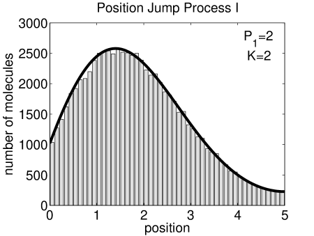
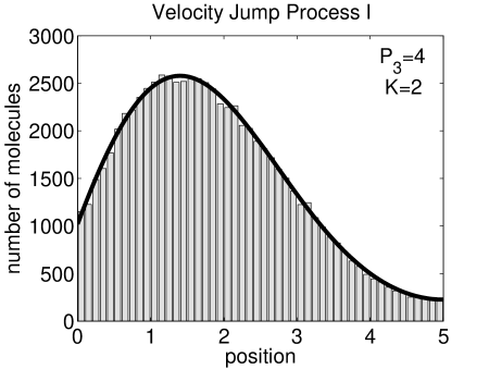
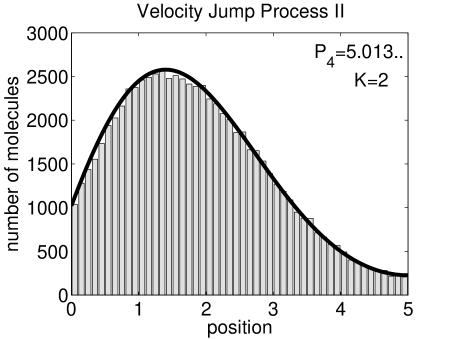
Figure 1: Stochastic simulations of four different diffusion models for $K=2$ and $D=1$. Probabilities of adsorption at partially adsorbing boundary $x=0$ were computed for each model according to formulas $(\ref{Kmod1})$, $(\ref{Kmod2})$, $(\ref{Kmod3})$ and $(\ref{Kmod4})$.

The initial condition was chosen as follows: we start with $100,000$ molecules in domain $[0,5]$. We put $75,000$ molecules to position $x=1$ and $25,000$ to position $x=2$ at time $t=0$. We plot the density profile at time $t=1$ in Figure 1. To do that, we divide the interval $[0,5]$ into 50 bins of length $0.1$ and we plot the number of molecules in each bin at time $t=1$ (histograms). We also plot the solution of diffusion equation (2) accompanied by Robin boundary condition (3) at $x=0$ and no-flux boundary condition at $x=L$. We see that all four models of diffusion give the same results provided that we choose the partially adsorbing probability accordingly.

To compute the simulation results from Figure 1, we also had to specify the additional parameters of the stochastic models. We used space step $h=0.1$ and time step $\Delta t=10^{-4}$ in Position Jump Process I. We used time step $\Delta t=10^{-4}$ in Position Jump Process II. We used speed $s=40$ and time step $\Delta t=10^{-5}$ in Velocity Jump Process I and we used friction coefficient $\beta=200$ and time step $\Delta t=10^{-6}$ in Velocity Jump Process II.

3.2 Consequences of the same probability of adsorption

Let us now consider the following boundary condition: whenever a molecule hits the boundary, it is adsorbed with probability $R$, and reflected otherwise. We can easily modify the computer codes which were used to compute stochastic simulation results from Figure 1 to incorporate this boundary condition: whenever the $i$-th molecule hits the boundary, we generate a random number $r_{i}$ uniformly distributed in $[0,1]$. If $r_{i}<R$, we remove the $i$-th molecule from the system. It means that the adsorbing condition which was stated in terms of $P_{1}$, $P_{2}$, $P_{3}$ and $P_{4}$ is replaced by the same condition expressed in terms of $R$. Choosing $R=0.05$ and the same parameters and initial condition as in Section 3.1, the stochastic simulation results at time $t=1$ are shown in Figure 2 (histograms obtained by dividing domain $[0,5]$ into 50 bins and plotting the number of molecules in each bin).

   

   

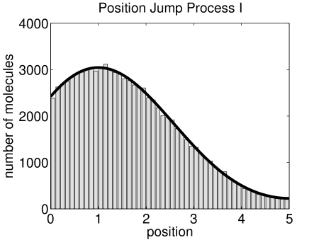
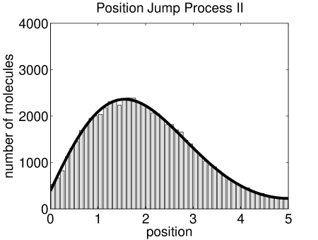
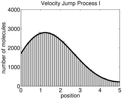
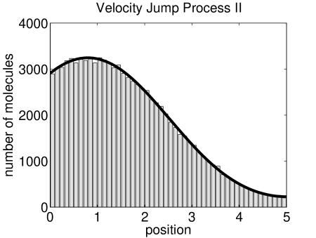
Figure 2: Stochastic simulations of four different diffusion models for $R=0.05$ and $D=1$ (histograms). Solid curves show the solution of the diffusion equation $(\ref{diffusionequation1D})$ accompanied by no-flux boundary condition at $x=5$ and Robin boundary condition $(\ref{RobinBD})$ at $x=0$ where the values of $K$ are computed according to formulas $(\ref{Kmod1})$, $(\ref{Kmod2})$, $(\ref{Kmod3})$ and $(\ref{Kmod4})$.

We clearly see that the results quantitatively differ. The reason is that the probability of adsorption scales with other parameters of simulations: namely with space step $h$ for Position Jump Process I, with time step $\Delta t$ for Position Jump Process II, with speed $s$ for Velocity Jump Process I and with friction coefficient $\beta$ with Velocity Jump Process II. The values of these scaling parameters were chosen as in Section 3.1. Namely, we used space step $h=0.1$ in Position Jump Process I, time step $\Delta t=10^{-4}$ in Position Jump Process II, speed $s=40$ in Velocity Jump Process I and friction coefficient $\beta=200$ in Velocity Jump Process II. Using these values, we can compute $P_{1}$, $P_{2}$, $P_{3}$ and $P_{4}$ which correspond to $R=0.05$. Moreover, we can use formulas $(\ref{Kmod1})$, $(\ref{Kmod2})$, $(\ref{Kmod3})$ and $(\ref{Kmod4})$ to compute the corresponding value of $K$ in Robin boundary condition (3). We obtain $K=0.5$ for Position Jump Process I, $K\doteq 5.64$ for Position Jump Process II, $K=1$ for Velocity Jump Process I and $K\doteq 0.28$ for Velocity Jump Process II. The solutions of diffusion equation (2) accompanied by no-flux boundary condition at $x=5$ and Robin boundary condition (3) at $x=0$ with the appropriate choice of $K$ are plotted in Figure 2 for comparison as solid curves. We see that the Robin boundary condition (3) at $x=0$ with the appropriate choice of $K$ gives the correct results when compared with stochastic simulations. Moreover, we also confirm that the same value of $R$ leads to the different values of $K$. Hence the boundary condition cannot be formulated in terms of one probability $R$. It has to be appropriately scaled as shown in Section 2.

To enable a direct comparison between models, we can slightly reformulate Position Jump Process I. The formulation from Section 2.1 was chosen in a way which is used in the stochastic reaction-diffusion approaches which are based on the reaction-diffusion master equation [10, 11]. In particular, no relation between $h$ and $\Delta t$ was given and the probability of partial adsorption had to be scaled with $h$. One can also formulate the position jump process on lattice as follows: we choose time step $\Delta t$ and space step $h=\sqrt{2D\,\Delta t}$. At each time step, the molecule jumps to the left with probability $1/2$ and to the right otherwise. This random walk can be accompanied with partially adsorbing boundary condition: whenever a molecule hits the boundary, it is adsorbed with probability $\widetilde{P}_{1}\sqrt{\Delta t}$, and reflected otherwise. This boundary condition leads to Robin boundary condition (3) with $K$ given by

$$K=\frac{\widetilde{P}_{1}\sqrt{D}}{\sqrt{2}}.$$

Comparing this formula with (9) or (13), we see that the Robin boundary condition is different for Position Jump Process I and Position Jump Process II even if we scale the adsorption probability with the same factor $\sqrt{\Delta t}$.

The velocity jump processes can also be further compared. To do this, let us note that the speed $s$ of a molecule can be estimated as $\sqrt{kT/m}$ where $k$ is the Boltzmann’s constant, $T$ is the absolute temperature and $m$ is the mass of a molecule. In particular, we get the relation $s=\sqrt{D\beta}$ which can be used to scale the boundary condition of Velocity Jump Process I in terms of $\sqrt{\beta}$ instead of $s$. Consequently, we can relate $P_{3}$ to $P_{4}$ by $P_{3}=P_{4}\sqrt{D}$. However, using this relation in (13), we obtain a different Robin boundary condition (3) than by using formula (17).

To summarize this section, it is possible to reformulate Position Jump Process I to have the adsorption probability of both position jump processes scaled as $P\sqrt{\Delta t}$. It is possible to relate $s$ to $\beta$ in Velocity Jump Process I to have the adsorption probability of both velocity jump processes scaled as $P/\sqrt{\beta}$. Then all four cases lead to Robin boundary condition (3) of the form

$$K=\alpha P\sqrt{D}$$ (19)

where $\alpha$ is model-dependent. Consequently, the boundary condition has to be chosen differently for each model to get the same value of $K$ in Robin boundary condition (3). One has to use formulas $(\ref{Kmod1})$, $(\ref{Kmod2})$, $(\ref{Kmod3})$ and $(\ref{Kmod4})$ as we showed in Section 3.1.

4 Mathematical analysis of stochastic models of diffusion

The goal of this section is to provide the justification of the results from Section 2. For each stochastic model, we show that the model leads to the diffusion equation (2) away from the boundary. Moreover, we derive the Robin boundary condition for each model.

4.1 Position Jump Process I

Let $p_{k}(t)$ be the probability of finding a molecule at mesh point $x_{k}=(2k-1)h/2$ where $k=1,2,\dots,M$. If $k\neq 1$, $k\neq M$, then $p_{k}$ satisfies

$$p_{k}(t+\Delta t)=\left(1-\frac{2D\Delta t}{h^{2}}\right)p_{k}(t)+\frac{D\Delta t}{h^{2}}\,\Big{(}p_{k+1}(t)+p_{k-1}(t)\Big{)}$$

which can be rewritten as

$$\frac{p_{k}(t+\Delta t)-p_{k}(t)}{\Delta t}=D\;\frac{p_{k+1}(t)+p_{k-1}(t)-2p_{k}(t)}{h^{2}}.$$

Passing to the limit $\Delta t\to 0$, $h\to 0$, we obtain the diffusion equation (2). The boundary condition at $x=0$ can be incorporated into the equation for $p_{1}(t)$ as

$$p_{1}(t+\Delta t)=\left(1-\frac{2D\Delta t}{h^{2}}\right)p_{1}(t)+\frac{D\Delta t}{h^{2}}\,\Big{(}p_{2}(t)+(1-P_{1}h)p_{1}(t)\Big{)}$$ (20)

which can be rewritten as

$$\sqrt{\Delta t}\,\,\frac{p_{1}(t+\Delta t)-p_{1}(t)}{\Delta t}=\frac{D\sqrt{\Delta t}}{h}\left(\frac{p_{2}(t)-p_{1}(t)}{h}-P_{1}\,p_{1}(t)\right).$$

Passing to the limit $\Delta t\to 0$, $h\to 0$ such that $\sqrt{\Delta t}/h$ is kept constant, we obtain (7).

4.2 Position Jump Process II

Position jump process (8) is a discretized version (Euler scheme) of the stochastic differential equation

$$X(t+dt)=X(t)+\sqrt{2D}\,dW(dt)$$ (21)

where $dW(dt)$ is the normal random variable with mean 0 and variance $dt$ (i.e. the propagator of the special Wiener process) and $D$ is the macroscopic diffusion constant. The diffusion equation (2) is the Fokker-Planck equation corresponding to the stochastic differential equation (21) and its derivation can be found in any standard textbook [17]. The derivation of Robin boundary condition (9) is more delicate and requires the application of asymptotic methods [2]. To do that, we consider the Position Jump Process II on the semiinfinite interval $[0,\infty)$ subject to the boundary condition (a)-(b) from Section 2.2. Let $p_{\Delta t}\equiv p_{\Delta t}(x,t):[0,\infty)\times\Delta t\,{\mathbb{N}}_{0}\to[0,\infty)$ be the probability density function of the discretized process (8) with the boundary condition (a)-(b), so that $p_{\Delta t}(x,i\Delta t)\mbox{d}x$ is the probability of finding a molecule in the interval $[x,x+\mbox{d}x]$ at time $t=i\Delta t.$ We have

$$p_{\Delta t}(x,t+\Delta t)=\int_{0}^{\infty}p(x,t+\Delta t\,|\,y,t)\,p_{\Delta t}(y,t)\,\mbox{d}y,$$ (22)

where $p(x,t+\Delta t\,|\,y,t)$ is the conditional probability distribution function of finding a molecule at point $x$ at time $t+\Delta t$ given that it is at point $y$ at time $t.$ There are two possible options to reach point $x$ at time $t+\Delta t$: either we use (8) only, i.e. $x=y+\sqrt{2D\,\Delta t}\;\zeta_{i}$; or we use the boundary condition $x=-y-\sqrt{2D\,\Delta t}\;\zeta_{i}$ with probability $1-P_{2}\sqrt{\Delta t}$. If the former is true, we have to take into account that some molecules are lost because of the Andrews and Bray boundary correction (b). Consequently, we have

$$p(x,t+\Delta t\,|\,y,t)=\frac{1}{\sqrt{4\pi D\,\Delta t}}\left(\left\{1-\exp\left[-\frac{xy}{D\Delta t}\right]P_{2}\sqrt{\Delta t}\right\}\exp\left[-\frac{(x-y)^{2}}{4D\,\Delta t}\right]+\right.$$

$$\left.\qquad+\;(1-P_{2}\sqrt{\Delta t})\exp\left[-\frac{(x+y)^{2}}{4D\,\Delta t}\right]\right)$$

$$=\frac{1}{\sqrt{4\pi D\,\Delta t}}\left(\exp\left[-\frac{(x-y)^{2}}{4D\,\Delta t}\right]+(1-2P_{2}\sqrt{\Delta t})\exp\left[-\frac{(x+y)^{2}}{4D\,\Delta t}\right]\right).$$

Thus (22) reads as follows

$$p_{\Delta t}(x,t+\Delta t)=$$

$$\int_{0}^{\infty}\frac{p_{\Delta t}(y,t)}{\sqrt{4\pi D\,\Delta t}}\left(\exp\left[-\frac{(x-y)^{2}}{4D\,\Delta t}\right]+(1-2P_{2}\sqrt{\Delta t})\exp\left[-\frac{(x+y)^{2}}{4D\,\Delta t}\right]\right)\mbox{d}y.$$ (23)

Away from the boundary, a steepest descent approximation to the integral as $\Delta t\to 0$ leads to the diffusion equation (2). However, as observed in [20], in the vicinity of the boundary, such a calculation needs to be modified: there is a boundary layer of width $\sqrt{\Delta t}$, and it is the solution in the boundary layer which determines the boundary condition of the diffusion equation. In the boundary layer, we change variables from $x$ to $\eta$ by setting $x=\sqrt{\Delta t}\,\eta$ and define the inner solution

$$p_{inner}(\eta,t)=p_{\Delta t}(\sqrt{\Delta t}\,\eta,t).$$

Expanding $p_{inner}$ in the powers of $\sqrt{\Delta t}$, we obtain

$$p_{inner}(\eta,t)\sim p_{i,0}(\eta,t)+\sqrt{\Delta t}\,p_{i,1}(\eta,t)+\Delta t\,p_{i,2}(\eta,t)+\dots.$$

Using this expansion in the integral equation (23) and comparing the terms of the same order, we obtain at $O(1)$ that $p_{i,0}$ is independent of $\eta$. At $O(\sqrt{\Delta t})$ we find that

$$p_{i,1}(\eta)=-2P_{2}\int_{0}^{\infty}\frac{p_{i,0}}{\sqrt{4\pi D}}\exp\left[-\frac{(\xi+\eta)^{2}}{4D}\right]\mbox{d}\xi$$

$$+\int_{0}^{\infty}\frac{p_{i,1}(\xi)}{\sqrt{4\pi D}}\left(\exp\left[-\frac{(\xi-\eta)^{2}}{4D}\right]+\exp\left[-\frac{(\xi+\eta)^{2}}{4D}\right]\right)\mbox{d}\xi.$$ (24)

Now by matching the inner boundary layer expansion with the outer expansion $p_{\Delta t}(x,t)\sim n(x,t)+\dots$, we find $p_{i,0}(t)=n(0,t)$ and

$$\lim_{\eta\to\infty}\frac{\partial p_{i,1}}{\partial\eta}(\eta,t)=\frac{\partial n}{\partial x}(0,t).$$ (25)

Thus to determine the boundary condition on $n$ at $x=0$ we need to determine the behaviour of $\partial p_{i,1}/\partial\eta$ as $\eta\to\infty.$ Differentiating (24) with respect to $\eta$, we obtain

$$\frac{\partial p_{i,1}}{\partial\eta}(\eta)=\frac{P_{2}\,p_{i,0}}{\sqrt{\pi D}}\exp\left[-\frac{\eta^{2}}{4D}\right]$$

$$+\int_{0}^{\infty}\frac{p_{i,1}(\xi)}{\sqrt{4\pi D}}\left(\frac{\xi-\eta}{2D}\exp\left[-\frac{(\xi-\eta)^{2}}{4D}\right]-\frac{\xi+\eta}{2D}\exp\left[-\frac{(\xi+\eta)^{2}}{4D}\right]\right)\mbox{d}\xi.$$

Using integration by parts, we obtain the integral equation

$$\frac{\partial p_{i,1}}{\partial\eta}(\eta)=\frac{P_{2}\,p_{i,0}}{\sqrt{\pi D}}\exp\left[-\frac{\eta^{2}}{4D}\right]$$ (26)

$$+\frac{1}{\sqrt{4\pi D}}\int_{0}^{\infty}\frac{\partial p_{i,1}}{\partial\eta}(\xi)\left(\exp\left[-\frac{(\xi-\eta)^{2}}{4D}\right]-\exp\left[-\frac{(\xi+\eta)^{2}}{4D}\right]\right)\mbox{d}\xi.$$

Let us define the function $g(\eta)$ by

$$g(\eta)=-\frac{P_{2}\,p_{i,0}}{\sqrt{\pi D}}\exp\left[-\frac{\eta^{2}}{4D}\right]+\frac{\partial p_{i,1}}{\partial\eta}(\eta).$$ (27)

Then (26) can be rewritten as

$$g(\eta)=\phi(\eta)+\frac{1}{\sqrt{4\pi D}}\int_{0}^{\infty}g(\xi)\left(\exp\left[-\frac{(\xi-\eta)^{2}}{4D}\right]-\exp\left[-\frac{(\xi+\eta)^{2}}{4D}\right]\right)\mbox{d}\xi$$ (28)

where

$$\phi(\eta)=\frac{P_{2}\,p_{i,0}}{\sqrt{8\pi D}}\,\exp\left[-\frac{\eta^{2}}{8D}\right]\left(\mathop{\mbox{erf}}\left[\frac{\eta}{\sqrt{8D}}\right]-\mathop{\mbox{erf}}\left[-\frac{\eta}{\sqrt{8D}}\right]\right)$$ (29)

and the error function is defined by

$$\mathop{\mbox{erf}}(\xi)=\frac{2}{\sqrt{\pi}}\int_{0}^{\xi}\exp\left[-\sigma^{2}\right]\mbox{d}\sigma.$$

The function $g(\eta)$ is defined for $\eta\geq 0$. Since $\phi(\eta)$ is odd function, we can define $g(\eta)$ for the negative values as an odd function too by setting $g(\eta)=-g(-\eta)$ for $\eta<0$. Then equation (28) can be simplified to

$$g(\eta)=\phi(\eta)+\frac{1}{\sqrt{4\pi D}}\int_{-\infty}^{\infty}g(\xi)\exp\left[-\frac{(\xi-\eta)^{2}}{4D}\right]\mbox{d}\xi.$$ (30)

The natural way to solve such an equation is to apply a Fourier transform, but we have to be slightly careful since the Fourier transform of $g$ does not exist in the classical sense ($g$ tends to a constant at infinity, so is not integrable). Defining

$$g_{+}(\eta)=g(\eta)\chi_{[0,\infty)}(\eta)\qquad g_{-}(\eta)=g(\eta)\chi_{(-\infty,0]}(\eta),$$

where $\chi_{[a,b]}$ is the characteristic function of the interval $[a,b]$ (that is, $\chi_{[a,b]}(\eta)=1$ if $a\leq\eta\leq b$ and zero otherwise), and applying the Fourier transform

$$\widehat{h}(k)=\int_{-\infty}^{\infty}h(\eta)\exp[ik\eta]\,\mbox{d}\eta$$

to equation (30), we obtain

$$\widehat{g_{+}}(k)+\widehat{g_{-}}(k)=\widehat{\phi}(k)+\left(\widehat{g_{+}}(k)+\widehat{g_{-}}(k)\right)\exp\left[-Dk^{2}\right].$$

Thus

$$\widehat{g_{+}}(k)+\widehat{g_{-}}(k)=\frac{\widehat{\phi}(k)}{1-\exp\left[-Dk^{2}\right]}.$$ (31)

This seems like one equation for the two unknowns $\widehat{g_{+}}(k)$ and $\widehat{g_{-}}(k)$, but in fact we know from their definitions that $\widehat{g_{+}}(k)$ is analytic for the imaginary part of $k$ positive, while $\widehat{g_{-}}(k)$ is analytic for the imaginary part of $k$ negative, and this tells us how to divide all the poles of the right-hand side between $\widehat{g_{+}}(k)$ and $\widehat{g_{-}}(k)$, except for the pole at the origin, which may appear in either $\widehat{g_{+}}(k)$ or $\widehat{g_{-}}(k)$. To divide this pole contribution up we note that since $g$ is odd, $\widehat{g_{+}}(k)=-\widehat{g_{-}}(-k)$, which implies that the coefficients of the odd powers of $k$ near zero are equal in $\widehat{g_{+}}(k)$ and $\widehat{g_{-}}(k)$, and that the coefficients of the even powers are zero.

Using (27) we have

$$\lim_{\eta\to\infty}\frac{\partial p_{i,1}}{\partial\eta}(\eta)=\lim_{\eta\to\infty}g(\eta)=\lim_{\eta\to\infty}\frac{1}{2\pi}\int_{-\infty}^{\infty}\widehat{g_{+}}(k)\exp[-ik\eta]\,\mbox{d}k,$$

where the inversion contour lies in the upper half-plane. Deforming the contour to $-i\infty$ we pick up residue contributions from each of the poles of (31) in the lower half plane. The only finite contribution as $\eta\rightarrow\infty$ arises from the pole at the origin. Since

$$\widehat{\phi}(k)\sim\frac{4i\sqrt{D}P_{2}p_{i,0}k}{\sqrt{\pi}}\mbox{ as }k\rightarrow 0,$$

we have

$$\widehat{g_{+}}(k)\sim\frac{2iP_{2}p_{i,0}}{\sqrt{\pi D}\,k}\mbox{ as }k\rightarrow 0,$$

so that

$$D\lim_{\eta\to\infty}\frac{\partial p_{i,1}}{\partial\eta}(\eta)=\frac{2P_{2}\,\sqrt{D}}{\sqrt{\pi}}\,p_{i,0}.$$

Using the matching condition (25) we therefore derive the Robin boundary condition (9) for the stochastic boundary condition (a)-(b). If we consider the boundary condition (a) only, equation (22) leads to the modified formula (23) where $2P_{2}$ is replaced by $P_{2}$. Thus the boundary layer method presented above gives in that case the Robin boundary condition (10), which differs from (9) by the factor of two.

4.3 Velocity Jump Process I

Using standard methods [12, 7], one can show that the density of molecules $n(x,t)$ satisfies the damped wave (telegrapher’s) equation

$$\frac{1}{2\lambda}\frac{\partial^{2}n}{\partial t^{2}}+\frac{\partial n}{\partial t}=\frac{s^{2}}{2\lambda}\frac{\partial^{2}n}{\partial x^{2}}.$$ (32)

The long time behaviour of (32) is described by the corresponding parabolic limit [22]. Using (11), we obtain that $n(x,t)$ satisfies (2) for times $t\gg\lambda^{-1}.$

Next, we derive the Robin boundary condition corresponding to (12). Let $p^{+}(x,t)$ be the density of molecules that are at $(x,t)$ and are moving to the right, and let $p^{-}(x,t)$ be the density of molecules that are at $(x,t)$ and are moving to the left. Then the density of molecules at $(x,t)$ is given by the sum $n(x,t)=p^{+}(x,t)+p^{-}(x,t),$ and the flux is $j(x,t)=s(p^{+}(x,t)-p^{-}(x,t))$. The stochastic boundary condition (12) implies

$$p^{+}(0,t)=\left(1-\frac{P_{3}}{s}\right)\,p^{-}(0,t).$$

This boundary condition can be written in terms of $n$ and $j$ as

$$\frac{1}{2}\left(n(0,t)+\frac{j(0,t)}{s}\right)=\left(1-\frac{P_{3}}{s}\right)\,\frac{1}{2}\left(n(0,t)-\frac{j(0,t)}{s}\right)$$

which implies

$$P_{3}\,n(0,t)=\left(\frac{P_{3}}{s}-2\right)\,j(0,t).$$

Since

$$j(0,t)\approx-D\frac{\partial n}{\partial x}(0,t),$$ (33)

we derive (13) in the limit $s\to\infty$.

4.4 Velocity Jump Process II

The random walk (14)-(15) is a discretized version of Langevin’s equation [3]. To derive the Robin boundary condition, we consider the behaviour of molecules in the semiinfinite interval $[0,\infty)$. The $i$-th molecule is described by two variables: its position $x_{i}(t)$ and its velocity $v_{i}(t)$. We compute the position $x_{i}(t+\Delta t)$ and velocity $v_{i}(t+\Delta t)$ from the position $x_{i}(t)$ and velocity $v_{i}(t)$ by (14)-(15) together with boundary condition (16) at $x=0$. Let $f(x,v,t)$ be the density of molecules which are at position $x$ with velocity $v$ at time $t$, so that $f(x,v,t)\,\delta x\,\delta v$ is number of molecules in interval $[x,x+\delta x]$ with velocities between $v$ and $v+\delta v$ at time $t$. Assuming that the change in velocity of the $i$-th molecule during the time step is $\Delta v$ (i.e. $\Delta v=v_{i}(t+\Delta t)-v_{i}(t)$), there are two possible options for the molecule to reach a point $x\geq 0$ with velocity $v$ at time $t+\Delta t$: either the molecule was at position $x_{i}(t)=x-(v-\Delta v)\Delta t$ with velocity $v_{i}(t)=v-\Delta v$ at time $t$; or at position $x_{i}(t)=-x+(v+\Delta v)\Delta t$ with velocity $v_{i}(t)=-v-\Delta v$ and was reflected according to (16). Both cases make sense only if $x_{i}(t)\geq 0$. Consequently, $f(x,v,t+\Delta t)$ can be computed from $f(\cdot,\cdot,t)$ by the integral equation

$$f(x,v,t+\Delta t)=\int_{v-x/\Delta t}^{\infty}f(x-(v-\Delta v)\Delta t,v-\Delta v,t)\,\psi(v-\Delta v;\Delta v)\,\mbox{d}\Delta v\;+$$ (34)

$$+\left(1-\frac{P_{4}}{\sqrt{\beta}}\right)\int_{-v+x/\Delta t}^{\infty}f(-x+(v+\Delta v)\Delta t,-v-\Delta v,t)\,\psi(-v-\Delta v;\Delta v)\,\mbox{d}\Delta v$$

where $\psi(w;\Delta v)$ is a distribution function of the conditional probability that the change in velocity during the time step is $\Delta v$ provided that $v_{i}(t)=w.$ Using (15), we obtain

$$\psi(w;\Delta v)=\frac{1}{\beta\sqrt{4\pi D\Delta t}}\exp\left[-\frac{(\Delta v+\beta w\Delta t)^{2}}{4\beta^{2}D\Delta t}\right].$$ (35)

Passing to the limit $\Delta t\to 0$, we obtain that $f(x,v,t)$ satisfies the Fokker-Planck equation [3]

$$\frac{\partial f}{\partial t}+v\frac{\partial f}{\partial x}=\beta\frac{\partial}{\partial v}\left(vf+\beta D\frac{\partial f}{\partial v}\right)$$ (36)

together with the boundary condition

$$f(0,v,t)=\left(1-\frac{P_{4}}{\sqrt{\beta}}\right)f(0,-v,t).$$ (37)

The density of molecules at the point $x$ and time $t$ is defined by

$$n(x,t)=\int_{\mathbb{R}}f(x,v,t)\,\mbox{d}v.$$ (38)

To derive the diffusion equation for $n$ and the corresponding Robin boundary condition we consider the limit in which $\beta\rightarrow\infty$ and rescale the velocity variable by setting

$$v=\eta\sqrt{\beta},\qquad\overline{f}(x,\eta,t)=f(x,v,t),$$

to give

$$\frac{1}{\beta}\frac{\partial\overline{f}}{\partial t}+\frac{1}{\sqrt{\beta}}\,\eta\frac{\partial\overline{f}}{\partial x}=\frac{\partial}{\partial\eta}\left(\eta\overline{f}+D\frac{\partial\overline{f}}{\partial\eta}\right).$$ (39)

We expand $\overline{f}$ in powers of $1/\sqrt{\beta}$ as

$$\overline{f}(x,\eta,t)=f_{0}(x,\eta,t)+\frac{1}{\sqrt{\beta}}\,f_{1}(x,\eta,t)+\frac{1}{\beta}\,f_{2}(x,\eta,t)+\dots.$$ (40)

Substituting (40) into (39) and equating coefficients of powers of $\beta$ we obtain

$$\frac{\partial}{\partial\eta}\left(\eta f_{0}+D\frac{\partial f_{0}}{\partial\eta}\right)=0,$$ (41)

$$\frac{\partial}{\partial\eta}\left(\eta f_{1}+D\frac{\partial f_{1}}{\partial\eta}\right)=\eta\frac{\partial f_{0}}{\partial x},$$ (42)

$$\frac{\partial}{\partial\eta}\left(\eta f_{2}+D\frac{\partial f_{2}}{\partial\eta}\right)=\eta\frac{\partial f_{1}}{\partial x}+\frac{\partial f_{0}}{\partial t}.$$ (43)

Solving equations (41)-(42), we obtain

$$f_{0}(x,\eta,t)=\varrho(x,t)\exp\left[-\frac{\eta^{2}}{2D}\right],$$ (44)

$$f_{1}(x,\eta,t)=-\frac{\partial\varrho}{\partial x}(x,t)\,\eta\exp\left[-\frac{\eta^{2}}{2D}\right]$$ (45)

where the function $\varrho(x,t)$ is independent of $\eta$. Substituting (44)-(45) into (43) gives

$$\frac{\partial}{\partial\eta}\left(\eta f_{2}+D\frac{\partial f_{2}}{\partial\eta}\right)=-\frac{\partial^{2}\varrho}{\partial x^{2}}\,\eta^{2}\exp\left[-\frac{\eta^{2}}{2D}\right]+\frac{\partial\varrho}{\partial t}\exp\left[-\frac{\eta^{2}}{2D}\right].$$

Integrating over $\eta$ gives the solvability condition

$$\frac{\partial\varrho}{\partial t}=D\frac{\partial^{2}\varrho}{\partial x^{2}}.$$

Using (38), we see that $\varrho(x,t)$ is proportional to density of individuals $n(x,t)$ for large $\beta$. Consequently, $n(x,t)$ satisfies the diffusion equation (2) for large $\beta$. Multiplying (37) by $v$ and integrating over $v$, we obtain

$$j(0,t)=-\frac{P_{4}}{\sqrt{\beta}}\int_{0}^{\infty}vf(0,-v,t)\,dv$$ (46)

where flux is defined by $j(0,t)=\int_{\mathbb{R}}vf(0,v,t)\,\mbox{d}v.$ Substituting (44)-(45) into (46), we derive the Robin boundary condition (17).

5 Boundary conditions for stochastic models of reaction-diffusion processes

In this section, we show that reactions in the solution do not change the boundary conditions from Section 2, i.e. the boundary conditions of stochastic models of the reaction-diffusion processes are determined by the corresponding diffusion model. First, we illustrate this fact numerically in Sections 5.1 and 5.2. In Section 5.1, we use the stochastic approach based on the reaction-diffusion master equation [10, 11], so that the corresponding diffusion model is the Position Jump Process I. In Section 5.2, we use the stochastic approach of Andrews and Bray [1], so that the corresponding diffusion model is the Position Jump Process II. Then, in Section 5.3, we provide mathematical justification of the fact that the presence of reactions in the solution does not influence the choice of the boundary condition.

5.1 Nonlinear reaction kinetics

We consider two chemicals $A$ and $B$ which diffuse in the domain of interest $[0,1]$ with diffusion constants $D_{A}$ and $D_{B}$, respectively, and which react according to Schnakenberg reaction kinetics [18]. The chemical $A$ is produced with a constant rate (from a suitable reactant which is supposed to be in excess) and degraded. The chemical $B$ is also produced with a constant rate. Moreover, $A$ and $B$ react according to the cubic reaction

$$2A+B\quad\mathop{\longrightarrow}^{k_{c}}\quad 3A$$ (47)

where $k_{c}$ is reaction constant. We use a partially adsorbing boundary condition at $x=0$ and a reflective boundary condition at $x=1$.

The stochastic simulation algorithm is based on the reaction-diffusion master equation [10, 11]. We divide the domain of interest into $M$ compartments of the length $h=1/M$ which are assumed to be well-mixed. In particular, one can use the classical Gillespie’s algorithm [9] to simulate stochastically the reactions in each compartment. The system is then described by two $M$-dimensional vectors $[A_{1},A_{2},\dots,A_{M}]$ and $[B_{1},B_{2},\dots,B_{M}]$ where $A_{i}$ (resp. $B_{i}$) denotes the number of molecules of chemical $A$ (resp. $B$) in the $i$-th compartment. The diffusion of chemicals is added to the system as another set of reactions–jumps between the neighbouring compartments with the rate $D_{A}/h^{2}$ (resp. $D_{B}/h^{2}$) [15]. In particular, the model of diffusion is equivalent to the Position Jump Process I.

We choose $M=50$ in what follows, i.e. $h=0.02$. Initially, we have $\omega=1000$ molecules of $A$ and $B$ in each compartment, i.e. $A_{i}=B_{i}=\omega$, $i=1,2,\dots,M$, at time $t=0$. The rate of production of $A$ is $2\omega$ molecules per compartment per unit of time. The rate of production of $B$ is $8\omega$ molecules per compartment per unit of time. The degradation rate of $A$ in the $i$-th compartment is proportional to $6A_{i}$ and $k_{c}$ is chosen to be $3\omega^{-2}$. Diffusion constants are $D_{A}=1$ and $D_{B}=0.1$. We implement the following boundary condition at $x=0$: whenever a molecule of chemical $A$ (resp. $B$) hits the boundary, it is adsorbed with probability $P^{A}_{1}h$ (resp. $P^{B}_{1}h$), and reflected otherwise. We choose $P^{A}_{1}=P^{B}_{1}=10$. We consider the reflective boundary condition for both chemicals at right boundary $x=1$. Number of molecules in each compartment at time $t=1$ are plotted in Figure 3 (histograms).

   

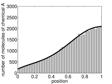
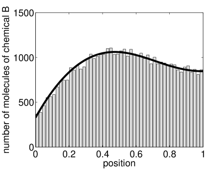
Figure 3: Stochastic simulations of the reaction-diffusion model of the Schnakenberg kinetics with the partially adsorbing boundary at $x=0$ (histograms). Panel on the left shows chemical $A$ and panel on the right chemical $B$. Solution of $(\ref{rd1})$-$(\ref{rd2})$ with the Robin boundary condition $(\ref{abRobinBD})$ at $x=0$ and no-flux boundary condition at $x=1$ is plotted as the solid line.

Since $\omega$ is chosen sufficiently large, we can compare the results of stochastic simulation with $\overline{A}=\omega a$ and $\overline{B}=\omega b$ where $a$, $b$ are the solution of the system of reaction-diffusion equations

$$\frac{\partial a}{\partial t}=D_{A}\,\frac{\partial^{2}a}{\partial x^{2}}+2-6a+3a^{2}\,b$$ (48)

$$\frac{\partial b}{\partial t}=D_{B}\,\frac{\partial^{2}b}{\partial x^{2}}+8-3a^{2}\,b$$ (49)

with Robin boundary conditions at $x=0$ given by (7), namely

$$\frac{\partial a}{\partial x}(0,t)=P^{A}_{1}\,a(0,t),\qquad\frac{\partial b}{\partial x}(0,t)=P^{B}_{1}\,b(0,t),$$ (50)

and with no-flux boundary conditions at right boundary $x=1$. The curves $\overline{A}=\omega a$ and $\overline{B}=\omega b$ at time $t=1$ are plotted in Figure 3 as solid lines for comparison. We see that the Robin boundary (7) which was derived for the corresponding diffusion model gives good results for the full reaction-diffusion simulation as well.

We note that the system (48)-(49) possesses a so-called Turing instability [13] if the values of the diffusion constants $D_{A}$ and $D_{B}$ are chosen to be sufficiently different. Our choice $D_{A}=1$ and $D_{B}=0.1$ falls in the regime in which the homogeneous solution $a=10/6$ and $b=48/50$ of (48)-(49) is stable. On increasing the ratio $D_{A}/D_{B}$ Turing patterns would develop, and we would observe solutions with multiple peaks (provided that the domain size is sufficiently large); see e.g. [15].

5.2 Spatially localized reactions

In some morphogenesis applications [19, 16], one assumes that some prepatterning in the domain exists and one wants to validate the reaction-diffusion mechanism of the next stage of the patterning of the embryo. In this section, we present an example motivated by this approach. We consider one-dimensional domain $[0,3]$ and we use the molecular based approach of Andrews and Bray [1], i.e. the diffusion model is given by Position Jump Process II. We choose a small simulation time step $\Delta t$. At each time step, a molecule is released at random points in the subinterval $[1,2]$ with probability $k_{p}\Delta t\ll 1$. Moreover, we assume that any molecule is degraded with probability $k_{d}\Delta t\ll 1$ during the simulation time step. Here, $k_{p}$ and $k_{d}$ are given constants. We implement the following boundary condition at $x=0$: whenever a molecule hits the boundary, it is adsorbed with probability $P_{2}\sqrt{\Delta t}$, and reflected otherwise. We consider the reflective boundary condition at right boundary $x=3$.

We start with no molecules in computational domain $[0,3]$ at time $t=0$. We choose diffusion constant $D=1$, time step $\Delta t=10^{-7}$, production rate $k_{p}=10^{5}$, degradation rate $k_{d}=1$ and adsorption probability constant $P_{2}=5$. To visualize the results, we divide the interval $[0,3]$ into 30 bins of length $0.1$ and we plot the number of molecules in each bin at time $t=1$ in Figure 4 (histogram). The results of the stochastic simulation

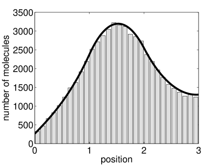
Figure 4: Stochastic simulations of the reaction-diffusion model with spatially localized reaction with the partially adsorbing boundary at $x=0$ (histogram). Solution of $(\ref{rd3})$ with Robin boundary condition $(\ref{RobinBD})$, with $K\doteq 5.642$, and with no-flux boundary condition at $x=3$, is plotted as the solid line.

can be compared with the solution of reaction-diffusion equation

$$\frac{\partial n}{\partial t}=D\,\frac{\partial^{2}n}{\partial x^{2}}+0.1\,k_{p}\chi_{[1,2]}-k_{d}n,$$ (51)

where $\chi_{[1,2]}$ is characteristic function of the interval $[1,2]$. Equation (51) is solved in the interval $[0,3]$ together with Robin boundary condition (3), with $K$ given by (9), and with no-flux boundary condition at $x=3$. Using $P_{2}=5$, formula (9) implies that $K\doteq 5.642$. The density profile $n(x,1)$ at time $t=1$ is plotted in Figure 4 as a solid line for comparison. We see that the Robin boundary condition (9), which was derived for the corresponding diffusion model, gives good results for the full reaction-diffusion simulation algorithm too.

5.3 Mathematical justification

Let us consider a system of $k$ chemicals diffusing and reacting in domain $[0,L]$. Let us suppose that the diffusion model is the Position Jump Process I, i.e. we use the stochastic approach based on the reaction-diffusion master equation [10, 11] as in Section 5.1. Let $p_{1}^{j}(t)$ (resp. $p_{2}^{j}(t)$) be the number of molecules of the $j$-th chemical, $j=1,2,\dots,k$, at the boundary mesh point $x_{1}=h/2$ (resp. at $x_{2}=3h/2$). If there are no reactions going on, then $p_{1}^{j}(t)$ and $p_{2}^{j}(t)$ are related according to (20). Introducing reactions at mesh point $x=h/2$, the boundary equation (20) is modified as follows

$$p_{1}^{j}(t+\Delta t)=\left(1-\frac{2D\Delta t}{h^{2}}\right)p_{1}^{j}(t)+\frac{D\Delta t}{h^{2}}\,\big{(}p_{2}^{j}(t)+(1-P_{1}h)p_{1}^{j}(t)\big{)}+\Delta tf(p_{1}^{1}(t),\dots,p_{1}^{k}(t))$$

where $f(p_{1}^{1}(t),\dots,p_{1}^{k}(t))$ is the sum of the rates of all reactions which modifies the $j$-th chemical. Following the same procedure as in Section 4.1, we find out that the additional term does not influence the boundary condition (it is $O(\Delta t)$ and only $O(\sqrt{\Delta t})$ terms have nonzero contribution to the Robin boundary condition). In particular, we conclude that the Robin boundary condition of the stochastic reaction-diffusion model is given by (7).

Next, let us consider the stochastic reaction-diffusion model of Andrews and Bray [1] which was used in Section 5.2. Let $p^{j}_{\Delta t}\equiv p^{j}_{\Delta t}(x,t):[0,\infty)\times\Delta t\,{\mathbb{N}}_{0}\to[0,\infty)$ be the density function of the $j$-th chemical species, so that $p^{j}_{\Delta t}(x,i\Delta t)\mbox{d}x$ is the number of $j$-th molecules in interval $[x,x+\mbox{d}x]$ at time $t=i\Delta t.$ If there are no reactions going on, then $p^{j}_{\Delta t}$ satisfies the formula (22). Introducing the reactions to the system, formula (22) is modified as follows:

$$p_{\Delta t}(x,t+\Delta t)=\int_{0}^{\infty}[1+O(\Delta t)]\,p(x,t+\Delta t\,|\,y,t)\,p_{\Delta t}(y,t)\,\mbox{d}y$$ (52)

where the additional $O(\Delta t)$ term corresponds to the reactions in the solution. As before, this term is of lower order (compared to $O(\sqrt{\Delta t})$ terms) and does not influence the Robin boundary condition. Consequently, the Robin boundary condition (3) is obtained with $K$ given by (9).

In this paper, we did not use the velocity jump processes to simulate stochastically the reaction-diffusion process. Velocity jump processes are generally more computationally intensive. However, they might be of use if one considers that only sufficiently fast molecules can actually react. Alternatively, one can use the approach based on binding/unbinding radii, as in the Andrews and Bray method [1], to incorporate higher order reactions to the velocity jump models of molecular diffusion. In any case, the reactions are adding again $O(\Delta t)$ terms and do not influence the boundary conditions, i.e. the boundary conditions of the stochastic reaction-diffusion models can be chosen as in the corresponding model of the diffusion only.

6 Conclusions and outlook

We have derived the correct boundary conditions for a number of stochastic models of reaction-diffusion processes. For each model, we related the (microscopic) probability of adsorption on the boundary with the (macroscopic) Robin (reactive) boundary condition (3). First, we studied several stochastic models of diffusion. We showed that each model is suitable for the description of the molecular diffusion far from the boundary. Moreover, we derived formulas (7), (9), (13) and (17) relating reactivity $K$ of the boundary with the parameters of the stochastic simulation algorithms. Then, we showed that the boundary conditions of stochastic models of reaction-diffusion processes are the same as for the corresponding model of diffusion only. We studied the stochastic approaches based on the reaction-diffusion master equation [10, 11] and on the Smoluchowski equation [1]. The main conclusion of this work is that a modeller can use any of the stochastic model of the diffusion from Section 2, provided that the adsorption probability on the reactive boundary is chosen according to the corresponding formula, i.e. (7), (9), (13) or (17), which is model-dependent.

We also presented the mathematical derivation of key formulas (7), (9), (13) and (17). We devoted the most space to the derivation of formula (9) which is (to our knowledge) a new mathematical result. Derivation of formulas (7) and (13) is simple and we included the mathematical arguments for completeness. The last formula (17) has already appeared in literature [14], though our derivation is more systematic.

It is interesting to note that in some applications, the reactivity of the boundary depends also on the geometrical constraints on the boundary. The binding sites on the surface (e.g. reactive groups or receptors) become full as the adsorption progresses. Moreover, attaching large molecules to a binding site can sterically shield the neighbourghing binding sites on the surface. For example, in [6, 4] we studied the chemisorption of polymers where the attachment of a long polymer molecule to the surface prevents attachment of other reactive polymers next to it. This steric shielding was modelled using random sequential adsorption [8]. In these models, an adsorption of one molecule to the surface is attempted per unit of time. To relate the time scale of random sequential adsorption algorithms with physical time, one should couple the theory of reactive boundaries presented here with algorithms which take the additional geometrical constraints on the boundary into account. This is an area of ongoing research [5].

Appendix. Robin boundary condition and chemistry

In this appendix, we show the relation between the Robin boundary condition (3) and the experimentally measurable chemical properties of the boundary. Let us consider a chemical diffusing in the domain $[0,L]$ which is adsorbed by boundary $x=0$ with some rate $\overline{K}$. This problem can be described by the reaction-diffusion equation

$$\frac{\partial n}{\partial t}=D\frac{\partial^{2}n}{\partial x^{2}}-\overline{K}n\,\delta(x),\qquad\mbox{for}\;x\in[0,L],\;t\geq 0,$$ (53)

together with no-flux boundary conditions, where $D$ is the diffusion constant and $\delta(x)$ a Dirac delta function. The term $\overline{K}n\,\delta(x)$ is a standard description of reaction kinetics, localized on the boundary. In the paper, we used an alternative description of the chemically adsorbing boundary, given by the diffusion equation (2) accompanied by the Robin boundary condition (3). It is interesting to note that the constant $K$ in (3) is actually equal to the experimentally measurable constant $\overline{K}$. To see this, we discretize (53) with space step $h$ and we denote $n_{0}(t)=n(h/2,t)$ and $n_{1}(t)=n(3h/2,t)$. Using a no-flux boundary condition (i.e. $n(-h/2,t)\equiv n(h/2,t)$), the discretization of (53) gives

$$\frac{\partial n_{0}}{\partial t}=D\frac{n_{1}-n_{0}}{h^{2}}-\overline{K}n_{0}\frac{1}{h}$$ (54)

which is equivalent to

$$\frac{\partial n_{0}}{\partial t}=D\frac{n_{1}-n_{0}+h\overline{K}n_{0}}{h^{2}}.$$ (55)

The same equation can be obtained by the discretization of the diffusion equation (2) together with the Robin boundary condition (3). Hence we showed that $K=\overline{K}$, i.e. the Robin boundary condition (3) is indeed the correct macroscopic description of the chemically reacting boundary.

References

References

- [1] S. Andrews and D. Bray, Stochastic simulation of chemical reactions with spatial resolution and single molecule detail, Physical Biology 1 (2004), 137–151.
- [2] C. Bender and S. Orszag, Advanced mathematical methods for scientists an engineers, McGraw-Hill book company, 1978.
- [3] S. Chandrasekhar, Stochastic problems in physics and astronomy, Reviews of Modern Physics 15 (1943), 2–89.
- [4] R. Erban and S. J. Chapman, On chemisorption of polymers to solid surfaces, 20 pages, to appear in Journal of Statistical Physics, available as arxiv.org/physics/0609029, 2006.
- [5] , What is the time scale of random sequential adsorption?, 4 pages, submitted to Physical Review Letters, available as arxiv.org/physics/0611252, 2006.
- [6] R. Erban, S. J. Chapman, K. Fisher, I. Kevrekidis, and L. Seymour, Dynamics of polydisperse irreversible adsorption: a pharmacological example, 22 pages, to appear in Mathematical Models and Methods in Applied Sciences (M3AS), available as arxiv.org/physics/0602001, 2006.
- [7] R. Erban and H. Othmer, From individual to collective behaviour in bacterial chemotaxis, SIAM Journal on Applied Mathematics 65 (2004), no. 2, 361–391.
- [8] J. Evans, Random and cooperative sequential adsorption, Reviews of Modern Physics 65 (1993), no. 4, 1281–1329.
- [9] D. Gillespie, Exact stochastic simulation of coupled chemical reactions, Journal of Physical Chemistry 81 (1977), no. 25, 2340–2361.
- [10] J. Hattne, D. Fagne, and J. Elf, Stochastic reaction-diffusion simulation with MesoRD, Bioinformatics 21 (2005), no. 12, 2923–2924.
- [11] S. Isaacson and C. Peskin, Incorporating diffusion in complex geometries into stochastic chemical kinetics simulations, SIAM Journal on Scientific Computing 28 (2006), no. 1, 47 – 74.
- [12] M. Kac, A stochastic model related to the telegrapher’s equation, Rocky Mountain Journal of Mathematics 4 (1974), no. 3, 497–509.
- [13] J. Murray, Mathematical Biology, Springer Verlag, 2002.
- [14] K. Naqvi, K. Mork, and S. Waldenstrom, Reduction of the Fokker-Planck equation with an adsorbing or reflecting boundary to the diffusion equation and the radiation boundary condition, Physical Review Letters 49 (1982), no. 5, 304–307.
- [15] L. Qiao, R. Erban, C. Kelley, and I. Kevrekidis, Spatially distributed stochastic systems: Equation-free and equation-assisted preconditioned computation, to appear in Journal of Chemical Physics, available as arxiv.org/q-bio/0606006, 2006.
- [16] G. Reeves, R. Kalifa, D. Klein, M. Lemmon, and S. Shvartsmann, Computational analysis of EGFR inhibition by Argos, Developmental biology 284 (2005), 523–535.
- [17] H. Risken, The Fokker-Planck Equation, methods of solution and applications, Springer-Verlag, 1989.
- [18] J. Schnakenberg, Simple chemical reaction systems with limit cycle behaviour, Journal of Theoretical Biology 81 (1979), 389–400.
- [19] O. Shimmi, D. Umulis, H. Othmer, and M. Connor, Faciliated transport of a Dpp/Scw heterodimer by Sog/Tsg leads to robust patterning of the Drosophila blastoderm embryo, Cell 120 (2005), no. 6, 873–886.
- [20] A. Singer, Z. Schuss, and D. Holcman, Partially reflected diffusion, 16 pages, preprint available as arxiv.org/math-ph/0606043, 2006.
- [21] A. Stundzia and C. Lumsden, Stochastic simulation of coupled reaction-diffusion processes, Journal of Computational Physics 127 (1996), 196–207.
- [22] E. Zauderer, Partial Differential Equations of Applied Mathematics, John Wiley & Sons, 1983.