An Efficient Algorithm for Solving the Phase Field Crystal Model

Abstract

We present and discuss the development of an unconditionally stable algorithm used to solve the evolution equations of the Phase Field Crystal (PFC) model. This algorithm allows for an arbitrarily large algorithmic time step. As the basis for our analysis of the accuracy of this algorithm, we determine an effective time step in Fourier space. We then compare our calculations with a set of representative numerical results, and demonstrate that this algorithm is an effective approach for the study of the PFC models, yielding a time step effectively 180 times larger than the Euler algorithm for a representative set of material parameters. As the PFC model is just a simple example of a wide class of density functional theories, we expect this method will have wide applicability to modeling systems of considerable interest to the materials modeling communities.

and

1 Introduction

The dynamics of a non-equilibrium system often results in highly complicated domain structures (microstructures). Typically, as time proceeds, the average size of these structures grows as a direct consequence of free-energy reduction: the interface is eliminated resulting in an increase in the size of homogeneous regions. Traditional non-equilibrium dynamics usually deals with the equilibrium states that are spatially uniform [1, 2, 3, 4], i.e., the stable phases are characterized by homogeneous values for the appropriate intensive thermodynamic variables. Classic, albeit quite simple, examples of models governing the evolution of such systems are the Cahn-Hilliard (CH) Equation for conserved systems [5] and Allen-Cahn (AC) Equation for non-conserved systems [6]. Examples are found in polymer mixtures [7], alloys [8, 9], liquid-crystals [10, 11], and in cosmology [12].

A model that has generated considerable recent interest is the Phase Field Crystal (PFC) Equation [13, 14], which is a conservative form of the familiar, non-conserved, Swift-Hohenberg (SH) Equation [15]. These systems differ from the CH and AC systems in that the stable phase is periodic. For SH models, the order parameter is viewed as capturing the inhomogeneities in a fluid associated with Rayleigh-Bénard convection. In the case of the PFC model, which is a simple version of more elaborate density functional theories of liquid/crystal interfaces [16, 17], the model captures features at the atomic scale, and thus contains highly detailed physical information about the system’s structure. Such models can describe many of the basic properties of polycrystalline materials that are realized during non-equilibrium processing.

The equations of motion governing these non-equilibrium phenomena are non-linear partial differential equations that cannot generally be solved analytically for random initial conditions. Therefore, computer simulations play an essential role in our understanding and characterization of non-equilibrium phenomena. The standard Euler integration is known to be unstable for time step $\Delta t$ above a threshold fixed by lattice spacing $\Delta x$ [18]. In CH and AC systems, to maintain an interfacial profile, the lattice spacing must be smaller than the interfacial width $\xi$, and in PFC and SH systems, $\Delta x$ must smaller than the periodicity selected by the system. Thus, the Euler update is inefficient, and in practice it is computationally costly to use to evolve large systems. Various computational algorithms [19, 20, 21] have been developed by increasing $\Delta t$ compared to the simplest Euler discretization. However, these methods still require a fixed time step, so they eventually become inefficient. Recently, unconditionally stable algorithms [22, 23, 24] were developed to overcome this difficulty for CH and AC Equations. These algorithms are a class of stable algorithms free of the fixed time step constraint for equations with a mix of implicit and explicit terms. While these algorithms allow for an increasing time step in CH systems as time proceeds, only a finite effective time step is possible for AC systems. A recent study [25], based on this unconditionally stable algorithm, demonstrated analytically that one can use an accelerated algorithm $\Delta t=At^{2/3}$ to drive the CH Equation, with the accuracy in correlation controlled by $\sqrt{A}$.

In this manuscript we apply this unconditionally stable algorithm to the PFC and SH Equations (Section $2$). In Section $3$ we establish the effectiveness of this approach through numerical studies of the algorithm, demonstrating that the algorithm is both efficient and accurate for solving PFC Equation. Finally, in Section $4$ we provide some concluding remarks.

2 Unconditionally stable algorithms for PFC Equation

In this section, we develop a class of unconditionally stable time stepping algorithms ($\Delta t$ taken arbitrarily large without the solution becoming unstable) to the PFC and SH Equations. Although the main purpose of this section is to study unconditionally stable algorithms for the PFC Equation, we include a parallel discussion of the SH Equation, as the methodology applies to both equations with only trivial differences.

2.1 Unconditionally Stable Finite Differences

Both the PFC and SH Equations start from a free energy functional that describes the configurational cost of periodic phases in contact with isotropic phases, and can be expressed as

$$F[\phi]=\int d{\bf x}\left\{\frac{1}{2}\phi\left[r+(1+\nabla^{2})^{2}\right]\phi+\frac{\phi^{4}}{4}\right\},$$ (1)

where the periodic order parameter $\phi({\bf x},t)$ has the wave number $k_{0}=1$ in equilibrium, and $r<0$ characterizes the quench depth. For the PFC equation, $r$ is proportional to the deviation of the temperature from the melting temperature $T_{M}-T$.

In the PFC model the order parameter (the density) is conserved, and thus the equation of motion is in the form of a continuity equation, $\partial\phi/\partial t=-\nabla\cdot{\bf j}$, with current ${\bf j}=-M\nabla(\delta F/\delta\phi)$, where $M$ is the mobility. Absorbing $M$ into the time scale, we obtain the dimensionless form of the PFC Equation

$$\frac{\partial\phi}{\partial t}=\nabla^{2}\frac{\delta F}{\delta\phi}=\nabla^{2}\left\{\left[r+(1+\nabla^{2})^{2}\right]\phi+\phi^{3}\right\}.$$ (2)

For the SH Equation, on the other hand, the order parameter is not conserved by the dynamics, and its evolution is postulated to have the the form

$$\frac{\partial\phi}{\partial t}=-\frac{\delta F}{\delta\phi}=-\left[r+(1+\nabla^{2})^{2}\right]\phi-\phi^{3}.$$ (3)

Eq. (3) has a simple dissipative form, where the rate of change of $\phi$ is proportional to the gradient (with an an $L^{2}$ inner product in functional space) of the free energy.

In order to obtain an unconditionally stable algorithm, we now follow methods previously developed for the CH and AC Equations [23, 24], and work out in some detail how to semi-implicitly parameterize the equation of motion. We begin by “splitting” the linear terms in the equation of motion into “forward” and “backward” pieces, both for Eq. (2):

$$\phi_{t+\Delta t}+\Delta t\nabla^{2}\left[(a_{1}-1)(r+1)\phi_{t+\Delta t}+2(a_{2}-1)\nabla^{2}\phi_{t+\Delta t}+(a_{3}-1)\nabla^{4}\phi_{t+\Delta t}\right]$$

$$= \phi_{t}+\Delta t\nabla^{2}\left[a_{1}(r+1)\phi_{t}+2a_{2}\nabla^{2}\phi_{t}+a_{3}\nabla^{4}\phi_{t}+\phi_{t}^{3}\right],$$ (4)

and for Eq. (3):

$$\phi_{t+\Delta t}-\Delta t\left[(a_{1}-1)(r+1)\phi_{t+\Delta t}+2(a_{2}-1)\nabla^{2}\phi_{t+\Delta t}+(a_{3}-1)\nabla^{4}\phi_{t+\Delta t}\right]$$

$$= \phi_{t}-\Delta t\left[a_{1}(r+1)\phi_{t}+2a_{2}\nabla^{2}\phi_{t}+a_{3}\nabla^{4}\phi_{t}+\phi_{t}^{3}\right].$$ (5)

The constants $a_{1}$, $a_{2}$ and $a_{3}$ control the degree of splitting. In order to find the constraints on these parameters that yield an unconditionally stable algorithms, a standard von Neumann linear stability analysis on Eq. (4) and Eq. (5) may be performed. The procedures are quite similar and the results are identical for these two equations. We will only show the details for the PFC model in next subsection.

2.2 Physical versus numerical instabilities

As was found in the analysis of Vollmayr-Lee and Rutenberg [23] for the CH equation, the PFC equation will be linearly unstable to perturbations for legitimate physical reasons. Specifically, the isotropic phase $\bar{\phi}$ can be metastable or unstable to the stable periodic (crystalline) phase [14] if the system is an undercooled liquid. This situation (which is precisely what we are interested in modeling) is established when $r+3\bar{\phi}^{2}<0$. This physical instability complicates our standard von Neumann stability analysis, as we wish to predict when our numerical methods will cause an instability that is unrelated to the physical instability resulting from the thermodynamic.

We can investigate the physical instability by a linear stability analysis on the equation of motion Eq. (2). We let $\phi=\bar{\phi}+\eta$, where $\bar{\phi}$ is a constant phase and $\eta$ is a small perturbation, and linearize the PFC Equation Eq. (2) in $\eta$ to get

$$\dot{\eta}_{t}=\nabla^{2}\left[(r+3\bar{\phi}^{2})+(1+\nabla^{2})^{2}\right]\eta_{t}.$$ (6)

This can be Fourier transformed to find

$$\dot{\eta}_{{\bf k},t}=-k^{2}\left[(r+3\bar{\phi}^{2})+(1-k^{2})^{2}\right]\eta_{{\bf k},t}.$$ (7)

The physical instability for the above equation occurs for

$$\mathbf{r_{k}}\equiv k^{2}\left[(r+3\bar{\phi}^{2})+(1-k^{2})^{2}\right]<0,$$ (8)

which reduces to $r+3\bar{\phi}^{2}<0$ with $k=1$ in the stable phase, as we indicated above.

Now we can proceed to analyze the numerical stability and determine the constraints for the splitting parameters. We linearize the general step Eq. (4) by substituting $\phi=\bar{\phi}+\eta$ and get

$$\eta_{t+\Delta t}+\Delta t\nabla^{2}\left[(a_{1}-1)(r+1)\eta_{t+\Delta t}+2(a_{2}-1)\nabla^{2}\eta_{t+\Delta t}+(a_{3}-1)\nabla^{4}\eta_{t+\Delta t}\right]$$

$$= \eta_{t}+\Delta t\nabla^{2}\left[a_{1}(r+1)\eta_{t}+2a_{2}\nabla^{2}\eta_{t}+a_{3}\nabla^{4}\eta_{t}+3\bar{\phi}^{2}\eta_{t}\right],$$ (9)

The Fourier transform of the above equation results in

$$\eta_{{\bf k},t+\Delta t}\left[1-\Delta tk^{2}\{(a_{1}-1)(r+1)-2(a_{2}-1)k^{2}+(a_{3}-1)k^{4}\}\right]$$

$$= \eta_{{\bf k},t}\left[1-\Delta tk^{2}\{a_{1}(r+1)-2a_{2}k^{2}+a_{3}k^{4}+3\bar{\phi}^{2}\}\right].$$ (10)

This can be re-expressed as

$$\eta_{{\bf k},t+\Delta t}[1+\Delta t\mathcal{L}_{\bf k}]=\eta_{{\bf k},t}[1+\Delta t\mathcal{R}_{\bf k}].$$ (11)

Note that $\mathbf{r_{k}}=\mathcal{L}_{\bf k}-\mathcal{R}_{\bf k}$. While we want to avoid numerical instability, the physical instability is to be expected during the dynamics, and will not lead to numerical problems. But, as we indicated above, both of the instabilities will be captured by a general von Neumann stability analysis. One manner of dealing with this is to recognize that a proper unconditionally stable algorithm will be stable if and only if $\mathbf{r_{k}}>0$ and should be unstable if and only if $\mathbf{r_{k}}<0$. The von Neumann stability criterion is $|\eta_{{\bf k},t+\Delta t}|<|\eta_{{\bf k},t}|$. We can express our restriction on the regime of von Neumann stability as

$$\left[1+\Delta t\mathcal{L}_{\bf k}\right]^{2} > \left[1+\Delta t\mathcal{R}_{\bf k}\right]^{2}\quad\mathrm{for}\ \mathbf{r_{k}}>0$$

$$\left[1+\Delta t\mathcal{L}_{\bf k}\right]^{2} < \left[1+\Delta t\mathcal{R}_{\bf k}\right]^{2}\quad\mathrm{for}\ \mathbf{r_{k}}<0.$$ (12)

The above inequalities can be rewritten as

$$\mathbf{r_{k}}\left[2+\Delta t(\mathcal{L}_{\bf k}+\mathcal{R}_{\bf k})\right] > 0\quad\mathrm{for}\ \mathbf{r_{k}}>0$$

$$\mathbf{r_{k}}\left[2+\Delta t(\mathcal{L}_{\bf k}+\mathcal{R}_{\bf k})\right] < 0\quad\mathrm{for}\ \mathbf{r_{k}}<0,$$

which, dividing by $\mathbf{r_{k}}$ can be reduced to a single inequality, $2+\Delta t(\mathcal{L}_{\bf k}+\mathcal{R}_{\bf k})>0$, which implies $0<\mathcal{L}_{\bf k}+\mathcal{R}_{\bf k}$ for arbitrarily large $\Delta t$, and we obtain

$$0<-k^{2}\left[(r+1)(2a_{1}-1)+3\bar{\phi}^{2}-2(2a_{2}-1)k^{2}+(2a_{3}-1)k^{4}\right],$$ (13)

which can be satisfied using the mode independent restrictions (and $r>-1$)

$$a_{1}<\frac{1}{2}-\frac{3\bar{\phi}^{2}}{2(r+1)},\ \ \ \ \ \ \ \ \ \ \ a_{2}\geq\frac{1}{2},\ \ \ \ \ \ \ \ \ \ \ a_{3}\leq\frac{1}{2}.$$ (14)

These are the constraints on the parameters $a_{1}$, $a_{2}$ and $a_{3}$ for unconditionally stable algorithms for all modes, for quenches in the range $-1<r<-3\bar{\phi}^{2}$. With these choices there is no threshold for $\Delta t$ in order to maintain numerical stability. The quantity $\Delta t$ is termed the algorithmic time step. We note that unconditional stability does not mean that the user of such algorithms may simply take as large a time step as is desired. Indeed, to obtain accurate physical results, there are additional restrictions on how large $\Delta t$ may be.

2.3 Effective time step

To determine how large a time step we may take, and still maintain an accurate solution, we calculate the Fourier space “effective time step”, as will be described below. We first note that when $a_{1}=a_{2}=a_{3}=1$, Eq. (4) corresponds to the traditional Euler update

$$\frac{\phi^{\prime}_{t+\Delta t}-\phi_{t}}{\Delta t_{Eu}}=\nabla^{2}\left\{\left[r+(1+\nabla^{2})^{2}\right]\phi_{t}+\phi_{t}^{3}\right\},$$ (15)

where $\phi^{\prime}_{t+\Delta t}$ denotes the field obtained after an Euler update on a previous field $\phi_{t}$, while we use the unprimed $\phi_{t+\Delta t}$ to denote the field obtained by unconditionally stable algorithm on $\phi_{t}$ throughout.

We now define the spatial Fourier transform of $\phi_{{\bf k},t}=\int d{\bf x}\e^{-i{\bf k}\cdot{\bf x}}\phi_{t}({\bf x})$. In Fourier space, writing $k^{2}\equiv|{\bf k}|^{2}$, the Euler update becomes

$$\frac{\phi^{\prime}_{{\bf k},t+\Delta t}-\phi_{{\bf k},t}}{\Delta t_{Eu}}=-k^{2}\left\{\left[r+(1-k^{2})^{2}\right]\phi_{{\bf k},t}+(\phi^{3})_{{\bf k},t}\right\},$$ (16)

where $(\phi^{3})_{{\bf k},t}=\int d{\bf x}\e^{-i{\bf k}\cdot{\bf x}}\phi_{t}^{3}({\bf x})$.

In Fourier space, the unconditionally stable algorithms Eq. (4) can be written in a form that is analogous to Eq. (16):

$$\frac{\phi_{{\bf k},t+\Delta t}-\phi_{{\bf k},t}}{\Delta t_{eff}^{PFC}(k,\Delta t)}=-k^{2}\left\{\left[r+(1-k^{2})^{2}\right]\phi_{{\bf k},t}+(\phi^{3})_{{\bf k},t}\right\},$$ (17)

where we define $k$-dependent effective time step by

$$\Delta t_{eff}^{PFC}(k,\Delta t)\equiv\frac{\Delta t}{1+\Delta tk^{2}[(r+1)(1-a_{1})+2k^{2}(a_{2}-1)+k^{4}(1-a_{3})]}$$ (18)

For SH Equation, the effective time step is

$$\Delta t_{eff}^{SH}(k,\Delta t)\equiv\frac{\Delta t}{1+\Delta t[(r+1)(1-a_{1})+2k^{2}(a_{2}-1)+k^{4}(1-a_{3})]}.$$ (19)

$\Delta t_{eff}(k,\Delta t)$ is an effective time step for a mode $k$, corresponding to an algorithmic time step $\Delta t$. Of particular interest in the case of periodic systems is the dominant mode (the lattice spacing in the PFC model), which, for the scaling choices made in Eq. (2) and Eq. (3) is simply $k_{0}=1$. Using the parameters employed in the simulations shown in the next section of $r=-0.025$, $a_{1}=0.45$, $a_{2}=0.5$, $a_{3}=0.5$, we obtain the dominant effective time step for both equations

$$\Delta t_{eff}(k_{0},\Delta t)=\frac{\Delta t}{1+29\Delta t/800}.$$ (20)

As $\Delta t=\infty$, we obtain the maximum dominant effective time step $\Delta t_{eff}(k_{0},\infty)=800/29\approx 27.6$. We see that a large algorithmic time step $\Delta t$ does not always translate into a significant amount of system evolution, as the effective time step always remains less than 28 for these parameter choices, no matter how large the algorithmic time step becomes. Thus, this value provides us with a useful bound on our exploration of just how large an algorithmic time step to take, and still obtain accurate results. For example, if we take algorithmic time steps that yields an effective time step $\Delta t_{eff}(k_{0},\Delta t)=\Delta t_{eff}(k_{0},\infty)/2=400/29$, then we find $\Delta t=800/29$. We demonstrate in the next section that this algorithm, when applied to the PFC Equation, realizes a significant speedup compared to the traditional Euler algorithm, while maintaining a controlled level of accuracy.

3 Numerical results

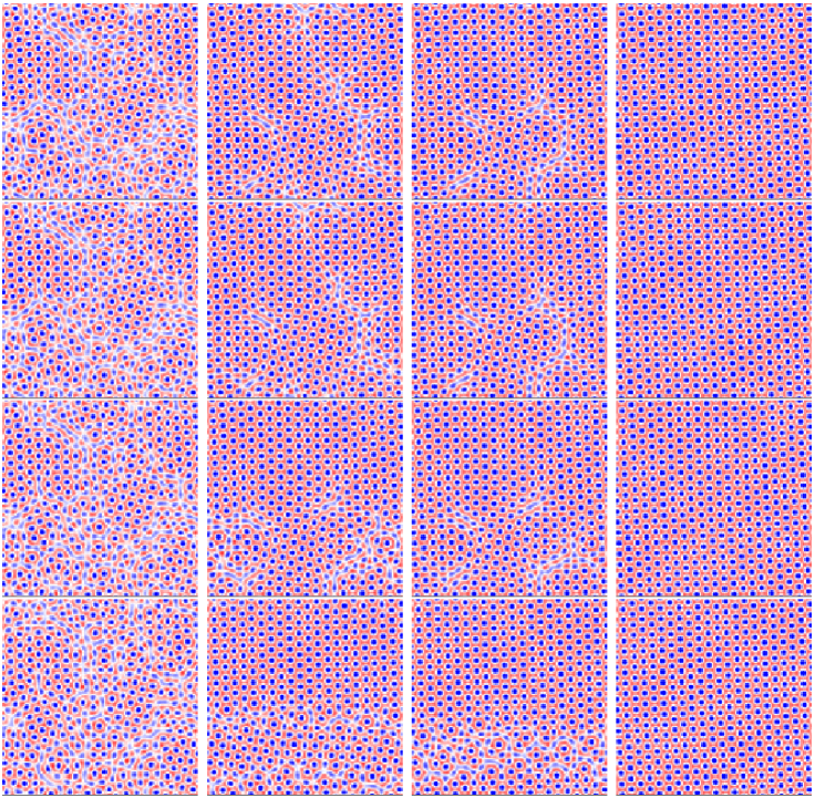
Figure 1: Snapshots of simulations of the PFC model. Time increases from left to right. The first row shows the field obtained using the Euler algorithm with $\Delta t_{Eu}=0.015$. The second to bottom rows show the fields obtained employing the unconditionally stable algorithms, when using algorithmic time steps of $\Delta t=3$, $\Delta t=10$, and $\Delta t=30$.

The simulations were performed in two-dimensions. Fig. 1 shows typical snapshots of simulations for the PFC model with parameters $\bar{\phi}=0.07$, $\Delta x=1.0$, and $L_{sys}=128$ with random initial conditions which corresponds to the liquid state. For comparison, all the simulations start with the same initial condition. In the Figure white regions indicate $\phi=\bar{\phi}$, red $\phi=\bar{\phi}+0.2$ and blue $\phi=\bar{\phi}-0.2$. The top row was obtained using the Euler algorithm $\Delta t_{Eu}=0.015$ at time steps $n=30000$, $n=60000$, $n=90000$, and $n=160000$. The second and lower rows were obtained using the unconditionally stable algorithm with (moving down) $\Delta t=3$, $\Delta t=10$, and $\Delta t=30$. For illustration and comparison purposes, we show the system snapshots at the same energy density as the top row — from left, the energy density $E=0.002374$, $E=0.002360$, $E=0.002357$, and $E=0.002350$ from the first to fourth column, respectively. We immediately see that, for the times and energies selected, there are no visible differences between the Euler update simulation and the unconditionally stable algorithm with $\Delta t=3$. However, there are visible differences between the Euler update and the simulations with $\Delta t>3$. We now wish to make these qualitative observations more quantitative.

Figure 2: A measure of the error $\sqrt{\langle(\phi_{eu}-\phi_{un})^{2}\rangle/\langle(\phi_{eu}-\bar{\phi})^{2}\rangle}$ versus the algorithmic time step $\Delta t$.

To study the accuracy, we compare simulations at the same energy density $E=0.002374$ (the first column in Fig. 1). We compute a measure of the error: $\sqrt{\langle(\phi_{eu}-\phi_{un})^{2}\rangle/\langle(\phi_{eu}-\bar{\phi})^{2}\rangle}$, where $\phi_{eu}({\bf x})$ denotes the fields obtained using Euler algorithm and $\phi_{un}({\bf x})$ denotes the fields obtained using the unconditionally stable algorithm. Fig. 2 shows a plot of the error versus a range of algorithmic time steps $\Delta t$. Fig. 2 indicates that, unsurprisingly, the accuracy increases as we decrease the algorithmic time step $\Delta t$. When $\Delta t\leq 3$, the error is below $5\%$. On the other hand, the error behavior in Fig. 2 for a large algorithmic time step tends to saturate, mirroring the saturation in the effective time step $\Delta t_{eff}$ for the dominant mode $k_{0}=1$.

Figure 3: A comparison between the theoretical dominant effective time step (solid line) and the numerical estimate of the same quantity (circle).

Fig. 3 shows a comparison between the dominant effective time step $\Delta t_{eff}(k_{0},\Delta t)$ in Eq. (20) and a numerical estimate of the same quantity. The numerical estimate is obtained by calculating $t_{Eu}^{tot}/n_{un}$, where $t_{Eu}^{tot}$ is the total time needed to reach the final state (a crystalline state without dislocations) using Euler algorithm and $n_{un}$ is the number of computer steps needed to reach the same state using unconditionally stable algorithms. We find good agreement for $\Delta t\leq 3$, while for $\Delta t>3$, the separation between the analytic and numerical expressions increases. While the agreement at small times steps in unsurprising, the curve provides a useful metric for the optimum algorithmic time step of $\Delta t\approx 3$, for the chosen parameters. When $\Delta t=3$, the ratio of the number of time steps needed to achieve a particular energy using the unconditionally stable versus Euler algorithm is approximately $180$ (the ratio of the dominant mode effective time step to the Euler time step). This is a substantial speedup, and requires minimal analysis to implement the technique.

4 Conclusions

In this paper, we have presented an unconditionally stable algorithm applicable to finite difference solutions of the the PFC Equation. We have demonstrated that a fixed algorithmic time step driving scheme may provide significant speedup, with a controlled level of accuracy, when compared with Euler algorithm. For the representative parameters chosen, a speedup of a factor of 180 was obtained. The analytical results and the numerical results are consistent with an effective time step analysis. Although this algorithm allows arbitrarily large algorithmic time steps, caution is indicated, as taking too large an algorithmic time step will yield inaccuracies with little improvement in the overall speedup of the calculation. This saturation in the speedup results from the details of how the system’s energy evolution (and its corresponding microstructural evolution) is governed by the effective time step, which saturates as the algorithmic time step increases. Thus, there is little advantage in too large an algorithmic time step. A method for obtaining a reasonable value for the algorithmic time step $\Delta t$ is suggested, in which a few test cases are run with different values of $\Delta t$ to see which one offers a good speedup and maintains the desired accuracy. The analytic form of the effective time step provides a useful guide for deciding how large a time step to select when trading off the obtainable speedup versus the loss of accuracy.

We expect the methodology developed in this paper could find extensive applications in a wide class of non-equilibrium systems. For example, it can be straightforwardly applied to the Swift-Hohenberg Equation, given its similarity with the Phase Field Crystal model. Additionally, the method also will apply to systems where there is a dominant mode realized at late times, such as is found in diblock co-polymers. This method should allow researchers to dramatically improve the computational efficiency associated with modeling the dynamics of materials systems.

5 Acknowledgments

We thank Andrew Reid and Daniel Wheeler for useful discussions.

References

- [1] J. S. Langer, in Solids far from Equilibrium, edited by C. Godrèche (Cambridge University Press, 1992), pp. 297.
- [2] A. J. Bray, Theory of phase-ordering kinetics, Adv. Phys. 43, 357 (1994).
- [3] J. D. Gunton, M. San Miguel and P. S. Sahni, in Phase Transitions and Critical Phenomena, Vol. 8, edited by C. Domb and J. L. Lebowitz (New York Academic Press, 1983) pp. 267.
- [4] H. Furukawa, Dynamic scaling assumption for phase separation, Adv. Phys., 34, 703 (1985).
- [5] J. W. Cahn and J. E. Hilliard, Free energy of a nonuniform system. I. Interface free energy, J. Chem. Phys. 28, 258 (1958).
- [6] S. M. Allen and J. W. Cahn, A microscopic theory for antiphase boundary motion and its application to antiphase domain coarsening, Acta Metall. 27, 1085 (1979).
- [7] P. Wiltzius and A. Cumming, Domain growth and wetting in polymer mixtures, Phys. Rev. Lett. 66, 3000 (1991).
- [8] R. F. Shannon, S. E. Nagler, C. R. Harkless and R. M. Nicklow, Time-resolved x-ray-scattering study of ordering kinetics in bulk single-crystal Cu3Au, Phys. Rev. B 46, 40 (1992).
- [9] B. D. Gaulin, S. Spooner and Y. Morii, Kinetics of phase separation in Mn0.67Cu0.33, Phys. Rev. Lett. 59, 668 (1987).
- [10] N. Mason, A. N. Pargellis and B. Yurke, Scaling behavior of two-time correlations in a twisted nematic liquid crystal, Phys. Rev. Lett. 70, 190 (1993).
- [11] I. Chuang, N. Turok and B. Yurke, Late-time coarsening dynamics in a nematic liquid crystal, Phys. Rev. Lett. 66, 2472 (1991).
- [12] P. Laguna and W. H. Zurek, Density of Kinks after a Quench: When Symmetry Breaks, How Big are the Pieces?, Phys. Rev. Lett. 78, 2519 (1997).
- [13] K. R. Elder, M. Katakowski, M. Haataja, and M. Grant, Modeling Elasticity in Crystal Growth, Phys. Rev. Lett. 88, 245701 (2002).
- [14] K. R. Elder and M. Grant, Modeling elastic and plastic deformations in nonequilibrium processing using phase field crystals, Phys. Rev. E 70, 051605 (2004).
- [15] J. Swift and P. C. Hohenberg, Hydrodynamic fluctuations at the convective instability, Phys. Rev. A 15, 319 (1977).
- [16] W. H. Shih, Z. Q. Wang, X. C. Zeng, and D. Stroud, Ginzburg-Landau theory for the solid-liquid interface of bcc elements, Phys. Rev. A 35, 2611 (1987).
- [17] K.-A. Wu, A. Karma, J. J. Hoyt, and M. Asta, Ginzburg-Landau theory of crystalline anisotropy for bcc-liquid interfaces, Phys. Rev. B 73, 094101 (2006).
- [18] T. M. Rogers, K. R. Elder and R. C. Desai, Numerical study of the late stages of spinodal decomposition, Phys. Rev. B 37, 9638 (1988).
- [19] Y. Oono and S. Puri, Study of phase-separation dynamics by use of cell dynamical systems. I. Modeling, Phys. Rev. A 38, 434 (1998).
- [20] L. Q. Chen and J. Shen, Applications of semi-implicit Fourier-spectral method to phase field equations, Comput. Phys. Commun. 108, 147 (1998).
- [21] J. Zhu, L. Q. Chen, J. Shen and V. Tikare, Coarsening kinetics from a variable-mobility Cahn-Hilliard equation: Application of a semi-implicit Fourier spectral method, Phys. Rev. E 60, 3564 (1999).
- [22] D. J. Eyre, in Computational and Mathematical Models of Microstructural Evolution, edited by J. W. Bullard et al. (The Material Research Society, Warrendale, PA, 1998), pp. 39-46.
- [23] B. P. Vollmayr-Lee and A. D. Rutenberg, Fast and accurate coarsening simulation with an unconditionally stable time step, Phys. Rev. E 68, 66703 (2003).
- [24] M. Cheng and A. D. Rutenberg, Maximally fast coarsening algorithms, Phys. Rev. E 72, 055701(R) (2005).
- [25] M. Cheng and J. A. Warren, Controlling the accuracy of unconditionally stable algorithms in Cahn-Hilliard Equation, cond-mat/0609354.