Low-energy effects in brane worlds: Liennard-Wiechert potentials and Hydrogen Lamb shift

Abstract

Testing extra dimensions at low-energies may lead to interesting effects. In this work a test point charge is taken to move uniformly in the 3-dimensional subspace of a (3+$n$)-brane embedded in a (3+$n$+1)-space with $n$ compact and one warped infinite spatial extra dimensions. We found that the electromagnetic potentials of the point charge match standard Liennard-Wiechert’s at large distances but differ from them close to it. These are finite at the position of the charge and produce finite self-energies. We also studied a localized Hydrogen atom and take the deviation from the standard Coulomb potential as a perturbation. This produces a Lamb shift that is compared with known experimental data to set bounds for the parameter of the model. This work provides details and extends results reported in a previous Letter.
Keywords: Brane worlds, Liennard-Wiechert, Hydrogen atom, Point charges.

1 Introduction

Spacetimes with more than three spatial dimensions have been attracting interest for long time. First proposals go back to Kaluza and Klein [1], in their attempt to unify electromagnetism with Einstein gravity by proposing a theory with a compact fifth dimension of a size of the order of the Planck length. Later on the emphasis shifted to a “brane world” picture [2, 3, 4] with our world being confined to a subspace of higher-dimensional spacetime. More recently it was put forward, inspired also in [5, 6], that at energy scales of the Standard Model matter cannot propagate into extra dimensions whilst gravity on the other hand can permeate all over. Within brane worlds extra dimensions may be compact but large [7, 8, 9], or infinite and warped [10, 11]. They have opened a rich and interesting phenomenological model-building aiming at solving long standing problems like the hierarchy and cosmological constant problem within high-energy physics [12, 13, 14], as well as testing models with observational data at the cosmological level [15].

We should stress at this point that to implement the brane scenario one looks for physical mechanisms which localize higher dimensional fields to a lower dimensional brane. Localization of gauge fields has turned out to be more difficult than that of scalar and spinors, however, some mechanisms have been developed in [16, 17, 18, 19]. The one in [16] is a particularly simple scenario that was probed to localize electromagnetic fields. It consists of a single (3+$n$)-brane embedded in a (3+$n$+1)-dimensional space containing $n$ compact extra dimensions and one infinite and warped. This is a (5+$n$)-dimensional brane world that we refer to as a Randall-Sundrum II model modified by $n$ extra compact dimensions (RSIIn). As for fermions some mechanisms have been developed in [20, 21, 22, 23, 24]. We shall combine some of these ideas for our purposes below.

It is generally assumed within brane models that relevant effects appear at high energies [12, 13, 14] whereas low-energy effects have no chance to become relevant. This is not necessarily the case since some high-precision tests may be sensible to such tiny effects or else, at worst, it may be possible to set bounds for the different parameters of the models [25, 26, 27]. In this paper we investigate two low-energy effects for RSIIn. The first one involves determining the electromagnetic potentials of point charge in uniform motion in a 3-dimensional subspace of the single (3+$n$)-brane. Considering that experiments in atomic physics are sensitive to small frecuency shifts down to 1 mHz [25, 26], one can in principle use the atom as an instrument to measure the anti-de Sitter radius $\epsilon$. The second problem we investigate is a Hydrogen atom, localized on the brane, where the binding electromagnetic field is just the one obtained in the first part. We have calculated the $2S_{1/2}-2P_{1/2}$ splitting coming from the presence of the extra dimensions that corresponds to the Lamb shift associated to QED. This has allowed us to set bounds for the parameter of the scenario, namely the anti-de Sitter radius or, equivalently, the tension of the brane. In the present work we provide details and extend some of the results of a previous Letter [28].

The paper is organized as follows. In section II we describe the RSIIn brane world and describe the localization mechanism for the electromagnetic and spinor fields. Section III is devoted to calculate the effective electromagnetic potentials for a test point charge in uniform motion thus providing details and generalizing the static results of [28]. In section IV the $2S_{1/2}-2P_{1/2}$ shift of a localized Hydrogen atom is calculated completely. Finally in section V we focus on the discussion of our results as well as some perspectives.

2 The scenario RSIIn

Now we describe the brane world we use in the present work. Looking for a localization mechanism for gauge fields as due to the gravity associated with the brane it was proved in [16] that the following setting would accomplish such task: A single (3+$n$)-brane embedded in a (3+$n$+1)-dimensional space so that space-time is ($5+n$)dimensional with $n$ compact dimensions and one infinite and warped. We call such a scenario RSIIn. Much as in the case of the Randall-Sundrum models to solve Einstein equations the brane tension and the negative bulk cosmological constant must be fine-tuned. The resulting metric is [16]

$$ds^{2}=a(y)^{2}\left(\eta_{\mu\nu}dx^{\mu}dx^{\nu}-\sum_{i=1}^{n}Rd\theta_{i}^{2}\right)-dy^{2},\qquad a(y)=e^{-\frac{|y|}{\epsilon}}\,,$$ (1)

where $\eta_{\mu\nu}$ is the four-dimensional Minkowski metric, $\theta_{i}$ $\in$ $[0,2\pi]$ are compact coordinates and $R_{i}$ are the sizes of the compact dimensions. $\epsilon$ is the anti-de Sitter radius.

Since our purpose is to study low energy-physics effects and hence the situation where electromagnetic fields and spinors are localized to a 3-dimensional subspace of the (3+$n$)-brane we next describe how this works in RSIIn.

2.1 Localization of the electromagnetic field

There has been extensive discussion about the localization of gauge fields in brane-worlds [16, 17, 19]. Here we just reproduce the proposal in [16] for the RSIIn scenario. Consider a gauge field $A_{M}$, with action

$$S_{g}=-\frac{1}{4}\int dx^{4}dy\prod\frac{d\theta_{i}}{2\pi R_{i}}\sqrt{g}g^{MP}g^{NQ}F_{MN}F_{PQ}\,.$$ (2)

For low-energies, hence $R_{i}$ small, and in the background (1), we truncate this action to the zero Kaluza-Klein modes of the compact $n$ dimensions. The effective 4-dimensional electromagnetic action turns out to be

$$S=-\frac{1}{4}\int_{-\infty}^{\infty}dy\,e^{-n\frac{|y|}{\epsilon}}\int dx^{4}\eta^{\mu\nu}\eta^{\lambda\rho}F_{\mu\lambda}F_{\nu\rho}\,.$$ (3)

Hence $A_{\mu}$ is normalizable, up to a normalization factor proportional to $\sqrt{\frac{n}{\epsilon}}$. If $n=0$ there is no localized gauge field, but for $n\geq 1$ the gauge field localizes on the brane and electrodynamics on it becomes 4-dimensional at large distances $l>\!\!>R_{i}$. We proceed next to discuss the spinor localization in RSIIn.

2.2 Localization of spinors

As in the case of the electromagnetic field in RSIIn, the observed 4-dimensional fields are the zero modes of higher dimensional ones. For explicit calculations we shall be considering $n$=1,2, namely 6- and 7-dimensional spacetime unless we specify otherwise, and hence 8-component spinors. The analysis should hold with the adequate generalizations for arbitrary $n$. We combine the localization mechanism of [22] designed to work in 5-dimensional spacetime for massive fermions with the projection analysis of [23, 29] that allows one to identify 4-component spinors out of the higher dimensional ones.

To begin with a domain wall is considered to be produced by some scalar field $\chi$. The domain wall separates two regions in the non-compact extra dimension $y$. Explicitly the region $\chi=-v$, $y<0$ separates from $\chi=v$, $y>0$. One introduces a Yukawa coupling between the spinor and the scalar $g\chi\bar{\psi}\psi$. For a given sign of the Yukawa coupling $g$ the zero modes have chirality defined. In general there is no dependence on the details of the profile of the scalar field across the wall. It turns out to be convenient to organize the chiral spinors into one field $\Psi$. The mass term is given by $\mu\bar{\Psi}\tau_{1}\Psi$. At low-energies, and hence small $R_{i}$, we truncate this action to the zero Kaluza-Klein modes of the compact $n$ dimensions. The resulting fermion action reads, after an adequate internal rotation [16],

$$S = \int dxdy\sqrt{g}\bar{\Psi}\left(\Gamma^{A}E_{A}^{M}\left[\partial_{M}+\Omega_{M}+ie^{(n)}A_{M}\right]+g\chi\tau_{1}+\mu\tau_{2}\right)\Psi,$$ (4)

$$\Psi = \left(\begin{array}[]{c}{\psi_{1}}\\ {\psi_{2}}\end{array}\right)\,.$$ (7)

Here $\psi_{1}$ and $\psi_{2}$ are spinors in ($5+n$)-dimensions and $\Omega_{M}=\frac{1}{2}\Omega_{M[AB]}\Sigma^{AB}$ is the spin conection, with generators $\Sigma_{AB}=\frac{1}{4}[\Gamma_{A},\Gamma_{B}]$. In what follows we restrict to the cases $n=1,2$ . In this way $\Gamma^{A}$ are six $8\times 8$ Dirac matrices. The Dirac equation which follows from this action in the background (1) has the form

$$\left[\Gamma^{A}E_{A}^{M}\left\{\partial_{M}+\Omega_{M}+ie^{(n)}A_{M}\right\}-g\chi(y)\tau_{1}-\mu\tau_{2}\right]\Psi=0\,.$$ (8)

Since the details of the profile of the scalar filed across the wall play no role for the localization of fields, we use an infinitely thin wall approximation. In this limit one has $g\chi(y)=gv$sign$(y)$. The components $\Omega_{A}$ are given in terms of the frames components through $\Omega_{A}=E_{A}^{M}\Omega_{M}$. Where the only non zero frames components are

$$E_{a}^{\mu}=\frac{1}{a(y)}\delta^{\mu}_{a},\qquad E^{y}_{\underline{y}}=1,\quad E^{\theta_{1}}_{\underline{\theta_{1}}}=\frac{1}{a(y)},\qquad E^{\theta_{2}}_{\underline{\theta_{2}}}=\frac{1}{a(y)}\,.$$ (9)

With $a=0,1,2,3$, the indices in the coordinate $\theta$ refer to $n=1,2$ and underlined indices refer to the orthonormal frame. The non-vanishing ones are

$$\Omega_{\mu}=\frac{1}{2}a(y)^{\prime}\Gamma_{y}\Gamma_{\mu},\quad\Omega_{\theta_{1}}=\frac{1}{2}a(y)^{\prime}\Gamma_{y}\Gamma_{\theta},\quad\Omega_{\theta_{2}}=\frac{1}{2}a(y)^{\prime}\Gamma_{y}\Gamma_{\theta}\,.$$ (10)

When $\mu\neq 0$ and $gv>1/2\epsilon$ there are no true localized modes but a metastable massive state [21, 22]. We assume such conditions hold for our $\chi$ and (8) becomes

$$\left[\frac{\Gamma^{\mu}\{\partial_{\mu}+e^{(n)}A_{\mu}\}}{a(y)}+\Gamma^{y}\partial_{y}-g\chi(y)\tau_{1}-\mu\tau_{2}\right]\Psi=0\,.$$ (11)

We proceed now by choosing Dirac matrices in the following form: $\Gamma_{\mu}=\gamma_{\mu}\otimes\sigma_{3}$, $\Gamma_{y}=\gamma_{5}\otimes\sigma_{3}$ and $\Gamma_{\theta}=1\otimes\sigma_{2}$. A convenient rearrangement for $\Psi$ is [23]:

$$\Psi=\phi(x)\otimes{\cal U}\otimes{\cal V}(y),\quad\Rightarrow\Gamma^{y}\otimes I_{2\times 2}\Psi_{R,L}=\pm\Psi_{R,L},\qquad{\cal U}=\binom{1}{0}\,.$$ (12)

Because of the presence of $\phi(x)$, from the point of view of 3-dimensional space, the spinor represents a quantum point-like particle. Now, the fundamental representation for $\Psi$ corresponds to the eigenvalues $+1$ and $-1$ for $\tau_{3}$, thus we use $\tau_{3}\Psi=\Psi$ as in [29]. In terms of $\Psi_{L,R}$ the equation(11) translates into a set of coupled equations,

$$\frac{\Gamma^{\mu}\{\partial_{\mu}-e^{(n)}A_{\mu}\}}{a(y)}\Psi_{L}+\partial_{y}\Psi_{R}-(g\chi(y)\tau_{1}+\mu\tau_{2})\Psi_{R}=0\,,$$ (13)

$$\frac{\Gamma^{\mu}\{\partial_{\mu}-e^{(n)}A_{\mu}\}}{a(y)}\Psi_{R}-\partial_{y}\Psi_{L}-(g\chi(y)\tau_{1}+\mu\tau_{2})\Psi_{L}=0\,.$$ (14)

By taking

$$\gamma^{\mu}\{\partial_{\mu}-e^{(n)}A_{\mu}\}\phi=m\phi$$ (15)

and after eliminating $\Psi_{L}$ in the system (13)-(14) one obtains a second order equation for ${\cal V}(y)$ that is given by

$$\left\{\frac{m^{2}}{a^{2}}+\partial_{y}^{2}-g\chi^{\prime}\tau_{1}-\kappa\,\mathrm{sign}(y)\partial_{y}+\kappa\,\mathrm{sign}(y)(g\chi\tau_{1}+\mu\tau_{2})+(g\chi\tau_{1}+\mu\tau_{2})^{2}\right\}{\cal V}(y)=0$$ (16)

¿From here on the same argument of [22] holds and there is a metastable state. Namely, for $\mu<<1/\epsilon$ one has

$$m=m_{0}-i\Delta$$ (17)

with

$$m_{0}=\left(1-\frac{1}{gv\epsilon}\right)\mu,\quad\Delta=m_{0}\left(\frac{m_{0}\epsilon}{2}\right)^{2gv\epsilon-1}\,\frac{\pi}{\left[\Gamma(gv\epsilon+1/2)\right]^{2}}$$ (18)

with $\Gamma(\dots)$ being the Gamma function. In the opposite regime, $\mu>>1/\epsilon$, one has

$$m_{0}=\mu,\quad\Delta=\frac{m_{0}}{2}\left(\frac{m_{0}}{2M}\right)^{2M\epsilon-1}\,e^{2M\epsilon},\quad M=\sqrt{(gv)^{2}+\mu^{2}}$$ (19)

Overall, for a given scalar field fulfilling the conditions above, that is to say $gv>1/2\epsilon$, it is possible to envisage a long life-time for the spinor to be localized on the brane. We assume this is the case and hence the role of the extra dimensions in RSIIn at low-energies for a localized Hydrogen atom we are interested in is reduced to an effective electromagnetic potential for a point-like proton which we describe in the following section.

3 Liennard-Wiechert potentials for a point particle

As a first step in the calculation of the energy levels corrections for Hydrogen atoms one has to find the effective electrostatic potential that replaces the Coulomb potential. In [28] we have presented the electrostatic potential produced by a point charge localized in the single brane. A uniformly moving 4D point charge source will be considered as follows

$$\sqrt{g}j^{\mu} = \sigma^{(5+n)}\ v^{\mu}\delta^{3}(\vec{x}-\vec{\mathrm{x}}(t))\delta(y-\mathrm{y}(t))\,,$$ (20)

$$\vec{\mathrm{x}}(t) = \vec{v}t\,,$$ (21)

$$\mathrm{y}(t) = \zeta\,.$$ (22)

Here $\sigma^{(5+n)}$ is the charge density and $v^{\mu}$ is the velocity of the source and $\zeta$ is a parameter that turns out to be useful in regularizing a delta product later on so we are interested at the end in the limit $\zeta\rightarrow 0$. For completeness we briefly recall the calculation leading to the photon Green’s function as given in the reference [16]. For the background (1) the Maxwell equations on the right to the brane yield

$${\cal O}\hat{A}^{\sigma}-e^{-n\frac{|y|}{\epsilon}}\hat{\partial}^{\sigma}\partial_{\mu}\hat{A}^{\mu}=-R^{-n}\sqrt{g}\,\,j^{\sigma},$$ (23)

$${\cal O}:=-e^{-(n+2)\frac{|y|}{\epsilon}}\partial^{2}_{y}+\frac{(n+2)}{\epsilon}e^{-(n+2)\frac{|y|}{\epsilon}}\,\mathrm{sign}(y)\partial_{y}+e^{-n\frac{|y|}{\epsilon}}\Box,$$ (24)

here we use the gauge $A^{y}=0$, $A^{\theta_{i}}=0$. $\hat{A}^{\nu}=\eta^{\nu\mu}A_{\mu}$ and $\Box$ is the 4D dalambertian. The term containing $\partial_{\mu}\hat{A}^{\mu}$ is pure gauge on the brane so we just drop it from now on. One now proceeds to solve (23) using the Green’s function approach, which satisfies

$${\cal O}G(y,y^{\prime})=\delta(x-x^{\prime})\delta(\theta-\theta^{\prime})\delta(y-y^{\prime})\,.$$ (25)

We solve this equation using the eigenfunction expansion for the Green’s function

$$G(x,x^{\prime},y,y^{\prime})=\int\frac{d^{4}k}{(2\pi)^{4}}e^{ik(x-x^{\prime})}\left[\frac{\phi_{0}(y)\phi_{0}(y^{\prime})}{k^{2}}+\int dm\frac{\phi_{m}(y)\phi_{m}(y^{\prime})}{k^{2}-m^{2}}\right].$$ (26)

Thus the corresponding eigenvalue equation for $\phi$ can be rewritten as

$$\left[-e^{-(n+2)\frac{|y|}{\epsilon}}\partial^{2}_{y}+\frac{(n+2)}{\epsilon}e^{-(n+2)\frac{|y|}{\epsilon}}\,\mathrm{sign}(y)\partial_{y}+e^{-n\frac{|y|}{\epsilon}}m^{2}\right]\phi(y)=0.$$ (27)

Notice that this equation is invariant under a change of sign in the coordinate $y$ and therefore it is enough to solve the equation in the region $y>0$ (on the right to the brane). Performing the change of variable $\xi=\epsilon e^{\frac{y}{\epsilon}}$ and redefining the function as $\phi=\xi^{\nu}\hat{\phi},\quad\nu=1+n/2$, one gets the Bessel equation

$$\partial_{\xi}^{2}\hat{\phi}_{m}+\frac{1}{\xi}\partial_{\xi}\hat{\phi}_{m}+\bigg{(}1-\frac{\nu^{2}}{\xi^{2}}\bigg{)}\hat{\phi}_{m} = 0\,.$$ (28)

When $m=0$ the solution has the form

$$\phi_{0}=\sqrt{\frac{n}{2\epsilon}}\,,\,\,\int_{-\infty}^{\infty}dy\,e^{-n\frac{|y|}{\epsilon}}\phi_{0}^{2}=1.$$ (29)

The weight factor $e^{-n\frac{|y|}{\epsilon}}$ comes from the Sturm-Liuville form of Eq. (27). In the case $m>0$ the normalized modes become

$$\phi_{m}=\sqrt{\frac{m\epsilon}{2}}\,\left(\frac{\xi}{\epsilon}\right)^{\nu}\left(\frac{N_{\nu-1}\left(m\epsilon\right)J_{\nu}\left(m\xi\right)-J_{\nu-1}\left(m\epsilon\right)N_{\nu}\left(m\xi\right)}{\sqrt{N^{2}_{\nu-1}\left(m\epsilon\right)+J^{2}_{\nu-1}\left(m\epsilon\right)}}\right),$$ (30)

fulfilling the boundary condition $\partial_{y}\phi_{m}(y)\big{|}_{y=0}=0$ as well as the normalization

$$\int_{-\infty}^{\infty}dye^{-n\frac{|y|}{\epsilon}}\phi_{m}(m\epsilon)\phi_{m^{\prime}}(m^{\prime}\epsilon)=\delta(m-m^{\prime})\,.$$ (31)

Performing the integration over $k$ in Eq.(26) yields the Green’s function on the brane

$$G_{R}(x-x^{\prime},y=0,y^{\prime}) = \frac{n}{2\epsilon}D_{0}(x-x^{\prime})+\int dm\phi_{m}(0)\phi_{m}(y^{\prime})D_{m}(x-x^{\prime}),$$ (32)

$$D_{0}(x-x^{\prime}) = \frac{\delta(\tau-r)}{4\pi r},\ \tau:=t-t^{\prime},\ r:=|\vec{x}-\vec{x}^{\prime}|,$$ (33)

$$D_{m}(x-x^{\prime}) = D_{0}(x-x^{\prime})+\frac{\theta(\tau-r)}{4\pi\sqrt{\tau^{2}-r^{2}}}mJ_{1}(m\sqrt{\tau^{2}-r^{2}}).$$ (34)

Here the first term is the contribution of the zero mode, $m=0$, the second term comes from the continuum of massive modes, $m>0$. The induced electromagnetic potential is obtained as usual by integrating the Green’s function with the source which in this case becomes

$$A^{\mu}(x,y=0)=-\int d^{4}x^{\prime}dy^{\prime}dm\frac{\theta[\tau-r]}{4\pi\lambda}mJ_{1}(m\lambda)\phi_{m}(0)\phi_{m}(y^{\prime})R^{-n}\sqrt{g}\,\,j^{\mu}(x^{\prime},y^{\prime})\,.$$ (35)

We have used equations (32)-(34), $\lambda:=\sqrt{\tau^{2}-r^{2}}$ and the completeness relation

$$\phi_{0}(y)\phi_{0}(y^{\prime})+\int dm\phi_{m}(y)\phi_{m}(y^{\prime})=\delta(y-y^{\prime})\,.$$ (36)

Notice that the eq. (35) is obtained by regularization of the product of $\delta$’s as follows: assume $\mathrm{y}(t)=\zeta$, with $\zeta$ a regulating parameter going to zero in the limit. This yields zero because of the delta product.

Now we focus on the evaluation (35). For low energies only small masses $m$ ($m<\!\!<1/\epsilon$) are relevant, and we obtain for the electromagnetic potential

$$A^{\mu}=-\frac{1}{R^{n}}\int dt^{\prime}dm\frac{v^{\mu}\theta[(t-t^{\prime})-|\vec{x}-\vec{\mathrm{x}}(t^{\prime})|]}{4\pi\Gamma(\nu-1)}\left(\frac{\epsilon}{2}\right)^{\nu-1}\sigma^{(5+n)}m^{\nu}J_{\nu}\left(\epsilon m\right)\frac{J_{1}\left(m\lambda\right)}{\lambda}\,.$$ (37)

For the evaluation of equation (37), there are two cases, whether ${n}$ is even or odd. We evaluate first the equation (37) for $n$ odd ($\nu$ half-integer). We use the relation

$$m^{l+1/2}J_{l+1/2}\left(m\epsilon\right)=\left(-1\right)^{l}\sqrt{\frac{2}{\pi}}\epsilon^{l+1/2}\left(\frac{d}{\epsilon d\epsilon}\right)^{l}\frac{\sin(m\epsilon)}{\epsilon},$$ (38)

and introduce (38) in (37) to integrate over $m$. So we easily find the result

$$A^{\mu}=\sqrt{\frac{2}{\pi}}\int_{-\infty}^{t_{*}}dt^{\prime}\frac{(-1)^{\nu-1/2}\theta[(t-t^{\prime})-|\vec{x}-\vec{\mathrm{x}}(t^{\prime})|]}{4\pi R^{n}\Gamma(\nu-1)\lambda}\sigma^{(5+n)}v^{\mu}\frac{\epsilon^{2\nu-1}}{2^{\nu-1}}\left(\frac{d}{\epsilon d\epsilon}\right)^{\nu-1/2}\frac{\theta[\lambda-\epsilon]}{\lambda\sqrt{\lambda^{2}-\epsilon^{2}}},$$ (39)

where $t_{*}$ satisfies $(t-t_{*})^{2}=\epsilon^{2}+|\vec{x}-\vec{\mathrm{x}}(t_{*})|^{2}$. It is possible to calculate the potential when the particle moves with uniform speed. We consider, for simplicity, the case when the motion takes place along the $x$ direction in the $xy$ plane, the solution is

$$A^{0}=\sqrt{\frac{2}{\pi}}\frac{(-1)^{\nu-1/2}\sigma^{(5+n)}\epsilon^{\nu}}{4\pi R^{n}\Gamma(\nu-1)}\frac{\epsilon^{2\nu-1}}{2^{\nu-1}}\left(\frac{d}{\epsilon d\epsilon}\right)^{\nu-1/2}\frac{\arctan{\left(\frac{\sqrt{y^{2}(1-v^{2})+(x-vt)^{2}}}{\epsilon\sqrt{1-v^{2}}}\right)}}{\epsilon\sqrt{y^{2}(1-v^{2})+(x-vt)^{2}}}.$$ (40)

For a static particle we have

$$A^{0}=\sqrt{\frac{2}{\pi}}\frac{(-1)^{\nu-1/2}}{4\pi R^{n}\Gamma(\nu-1)}\sigma^{(5+n)}\frac{\epsilon^{2\nu-1}}{2^{\nu-1}}\left(\frac{d}{\epsilon d\epsilon}\right)^{\nu-1/2}\frac{1}{2r\epsilon}\left[\arctan{\left(\frac{r}{\epsilon}\right)}\right],\quad r=|\vec{x}|.$$ (41)

For the case of $n$ even ($\nu$ integer), we can use the relation

$$m^{\nu}J_{\nu}\left(m\epsilon\right)=(-1)^{\nu}\epsilon^{\nu}\left(\frac{d}{\epsilon d\epsilon}\right)^{\nu}J_{0}\left(m\epsilon\right)$$ (42)

and integrating over $m$ the electromagnetic potential can be rewritten as

$$A^{\mu}=-\int_{-\infty}^{t_{*}}dt^{\prime}\frac{\theta[(t-t^{\prime})-|\vec{x}-\vec{\mathrm{x}}(t^{\prime})|]}{4\pi R^{n}\Gamma(\nu-1)}\frac{\sigma^{(5+n)}v^{\mu}(-1)^{\nu}}{\lambda}\frac{\epsilon^{2\nu-1}}{2^{\nu-1}}\left(\frac{d}{\epsilon d\epsilon}\right)^{\nu-1}\frac{\delta[\lambda-\epsilon]}{\epsilon\lambda}.$$ (43)

The electromagnetic potential for a point particle that moves with uniform speed is given by

$$A^{\mu}=-\frac{(-1)^{\nu+1}\epsilon^{2\nu}}{4\pi R^{n}\Gamma(\nu-1)2^{\nu-1}}{\left(\frac{d}{\epsilon d\epsilon}\right)}^{\nu-1}\frac{\sigma^{(5+n)}v^{\mu}}{\epsilon^{2}(\sqrt{\epsilon^{2}+|\vec{x}-\vec{\mathrm{x}}(t_{*})|^{2}}-\hat{n}\cdot\vec{v}|\vec{x}-\vec{\mathrm{x}}(t_{*})|)}\,,$$ (44)

where $\hat{n}=[\vec{x}-\vec{\mathrm{x}}(t_{*})]/[|\vec{x}-\vec{\mathrm{x}}(t_{*})|]$.

For the static particle we have the following potential

$$A^{0}=\frac{(-1)^{\nu+1}}{4\pi R^{n}\Gamma(\nu-1)}\frac{\epsilon^{2\nu-1}}{2^{\nu-1}}\left(\frac{d}{\epsilon d\epsilon}\right)^{\nu-1}\frac{\sigma^{(5+n)}\theta(\sqrt{\epsilon^{2}+r^{2}}-r^{2})}{\epsilon^{2}\sqrt{\epsilon^{2}+r^{2}}},\quad r=|\vec{x}|.$$ (45)

Let us present the above results for $A^{0}(x,t)=A^{0}(r,t)$ for $n=1$ and $n=2$.

$n=1$:
Liennard-Wiechert

$$A^{0}=\frac{e^{(n=1)}_{\mathrm{eff}}}{\epsilon}\left\{\frac{1}{\sqrt{1-v^{2}}\left(1+\frac{y^{2}(1-v^{2})+(x-vt)^{2}}{\epsilon^{2}(1-v^{2})}\right)}+\frac{\arctan{\left(\frac{\sqrt{y^{2}(1-v^{2})+(x-vt)^{2}}}{\epsilon\sqrt{1-v^{2}}}\right)}}{\frac{\sqrt{y^{2}(1-v^{2})+(x-vt)^{2}}}{\epsilon}}\right\},$$ (46)

Static case

$$A^{0}=\frac{e^{(n=1)}_{\mathrm{eff}}}{\epsilon}\left\{\frac{1}{1+\tilde{x}^{2}}+\cfrac{\arctan\left(\tilde{x}\right)}{\tilde{x}}\right\},\quad\tilde{x}=\frac{r}{\epsilon},\quad e^{(n=1)}_{\mathrm{eff}}:=\frac{\sigma^{(6)}}{2R\pi\epsilon^{2}}.$$ (47)

$n=2$:
Liennard-Wiechert

$$A^{0} = \frac{e^{(n=2)}_{\mathrm{eff}}}{\epsilon}\left\{\frac{1}{\left[\sqrt{1+R(t_{*})^{2}}-\hat{n}\cdot\vec{v}R(t_{*})\right]}+\frac{\left(1-|\vec{v}|^{2}\right)}{2\left[\sqrt{1+R(t_{*})^{2}}-\hat{n}\cdot\vec{v}R(t_{*})\right]^{3}}\right\},$$ (48)

$$R(t_{*}) = \frac{|\vec{x}-\vec{\mathrm{x}}(t_{*})|}{\epsilon}$$ (49)

Static case

$$A^{0}=\frac{e^{(n=2)}_{\mathrm{eff}}}{\epsilon}\left\{\frac{1}{\sqrt{1+\tilde{x}^{2}}}+\frac{1}{2\left(1+\tilde{x}^{2}\right)^{3/2}}\right\},\quad e^{(n=2)}_{\mathrm{eff}}:=\frac{\sigma^{(7)}}{R^{2}\pi\epsilon}.$$ (50)

Our electrostatic potentials for $n=1,2$ are consistent with the Coulomb potential at long distances and they preserve spherical symmetry. Remarkably these electrostatic potentials are finite at the position of the charge. See Fig. (1). The finite character of our effective electrostatics potentials allows to maintain the idea of an effective 3D point particle.

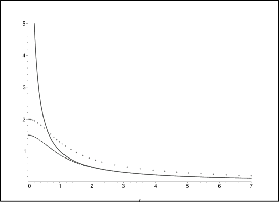
Figure 1: Effective electrostatic potential for the point particle multiplied, respectively, by the factor $4\pi\epsilon_{0}/e$ for the standard 4D case and $4\pi\epsilon_{0}/e_{eff}$ for $n=1,2$ compact extra dimensions. $e_{eff}$ is the effective charge of the particle in the latter case. The continuous curve represents standard 4D Coulomb potential, the crosses correspond to $n=1$ whereas the dashes are associated with $n=2$. Units are such that $\epsilon=1$.

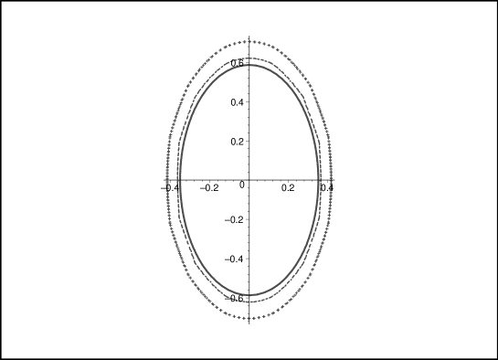
Figure 2: Equipotential surfaces of the effective Liennard-Wiechert potentials for the point particle. The continuous curve represents the standard 4D case, the dashes $n=1$ and the crosses $n=2$. A value of the potential of 2.98 was used for the potential multiplied by the factor $4\pi\epsilon_{0}/e$ for the standard 4D case and $4\pi\epsilon_{0}/e_{eff}$ with $e_{eff}$ for the effective charge of the particle for $n=1,2$ compact extra dimensions. Units are such that $\epsilon=1$ and the speed of the particle is $v=0.9$ along the horizontal axis.

Fig. (2) shows the effective electromagnetic and standard 4D Liennard-Wiechert potentials. In polar coordinates with the origin at the particle’s position at the present time and $R(t_{*})$ given by the solution of

$$R^{2}(1-v^{2})+2v\rho\sqrt{\epsilon^{2}+R^{2}}\,\cos\theta-\rho^{2}=0.$$ (51)

So $R$ can take on the values

$$R_{1,2} = \frac{\sqrt{\rho^{2}(2v^{2}\cos^{2}\theta-v^{2}+1)\pm 2v\rho\Sigma\cos\theta}}{1-v^{2}},$$ (52)

$$\Sigma := \sqrt{\rho^{2}(v^{2}\cos^{2}\theta-v^{2}+1)+\epsilon^{2}(1-v^{2})^{2}}$$ (53)

In the electromagnetic potential Eq. (48) $R(t_{*})=R_{1}$ for $\theta\in[\pi/2,3\pi/2]$ and $R(t_{*})=R_{2}$ for $\theta\in[-\pi/2,\pi/2]$.

4 Hydrogen Lamb shift

In this section we calculate the possible corrections to the energy levels for a Hydrogen atom caused by the existence of extra dimensions in RSIIn. The effective four-dimensional Dirac equation is given by

$$\left(i\gamma^{\mu}\partial_{\mu}-e^{(n)}\gamma^{0}A_{0}-m\right)\phi=0.$$ (54)

Here $A^{0}$ is given by (47) in the case of one compact extra dimension and (50) for two compact extra dimensions and $e^{(n)}$ stands for the electron charge as coming from $5+n$ dimensional spacetime. Given the complexity of the effective electrostatic potential we calculate the energy shifts by means of perturbation theory to first order.

We consider first the $n=1$ compact extra dimension case. Expanding the electrostatic potential (47) around the Coulomb potential, ie $r>\!\!>\epsilon$, gives

$$e^{(n=1)}A_{0}\approx-\alpha\left\{\frac{1}{r}-\frac{4}{3\pi}\frac{\epsilon^{3}}{r^{4}}\right\}\,,\quad\alpha:=e^{(n=1)}_{{\mathrm{eff}}}e^{(n=1)}.$$ (55)

¿From here on we shall assume $\alpha=\alpha_{\mathrm{QED}}$ in order to compare with experimental data. Within the present approximation the stationary part of Dirac equation (54) can be rewritten as

$$E\phi = ({\mathbf{H}}_{D}+{\mathbf{H}})\phi,$$ (56)

$${\mathbf{H}}_{D} = {\boldsymbol{\alpha}}\cdot{\mathbf{p}}+m{\boldsymbol{\beta}}-\frac{\alpha}{r},$$ (57)

$${\mathbf{H}}^{(n=1)} = \frac{4\alpha}{3}\frac{\epsilon^{3}}{r^{4}},$$ (58)

where the eigenvalue $E$ is the energy and ${\mathbf{H}}_{D}$ is the Dirac Hamiltonian for the unperturbed Hydrogen atom and ${\mathbf{H}}^{(n=1)}$ is the perturbation. Also $\boldsymbol{\alpha},\boldsymbol{\beta}$ are Dirac’s matrices. For the solutions to the Dirac equation in a Coulomb potential with energy $E$ and angular momentum quantum numbers ($\kappa\bar{m}$) we take the following form [30]

$$\phi_{\bar{n}\kappa\bar{m}}=\frac{1}{r}\begin{pmatrix}G_{\bar{n}\kappa\bar{m}}(r)\Omega_{\kappa,\bar{m}}(\vartheta,\varphi)\\ iF_{\bar{n}\kappa\bar{m}}(r)\Omega_{\kappa,\bar{m}}(\vartheta,\varphi)\end{pmatrix}.$$ (59)

Here $\bar{n}=0,1,\dots$ is the principal quantum number. In the Coulomb case the functions $F$ and $G$ are related to the confluent hypergeometric functions and $\Omega_{\kappa\bar{m}}(\vartheta,\varphi)$ are the spherical spinors. The latter are eigenfunctions of $K=-1-\vec{\sigma}\cdot\vec{L}$ with eigenvalues $\kappa=\mp(j+1/2)$ for $j=l\pm 1/2$. They satisfy the orthogonality relations

$$\int_{0}^{\pi}\sin\vartheta d\vartheta\int_{0}^{2\pi}d\varphi\Omega^{{\dagger}}_{\kappa^{\prime}\bar{m}^{\prime}}\Omega_{\kappa\bar{m}}=\delta_{\kappa^{\prime},\kappa}\delta_{\bar{m}^{\prime},\bar{m}}.$$ (60)

The corresponding energy eigenvalues are

$$E_{\bar{n}\kappa}=\frac{m}{\sqrt{1+\cfrac{\alpha^{2}}{(\gamma+\bar{n}-|\kappa|)^{2}}}}\;,\;\;\gamma=\sqrt{\kappa^{2}-\alpha^{2}}\,.$$ (61)

When calculating the energy shifts to lowest order in $\alpha$ the contribution of $F$ can be neglected. The energy shifts are determined by the matrix elements of the perturbation

$$H_{(\bar{n}\kappa\bar{m})(\bar{n}^{\prime}\kappa^{\prime}\bar{m}^{\prime})}=\int drr^{2}d\Omega\phi_{\bar{n}\kappa\bar{m}}^{{\dagger}}{\mathbf{H}}\phi_{\bar{n}^{\prime}\kappa^{\prime}\bar{m}^{\prime}}.$$ (62)

We want to calculate the energy split between the $2S_{1/2}$ and $2P_{1/2}$ states, $\Delta E^{(n)}:=\delta E^{(n)}_{2S_{1/2}}-\delta E^{(n)}_{2P_{1/2}}$, due to the presence of the $n$ compact extra dimensions and compare it with the experimental value for the Lamb shift $\Delta E^{\mathrm{Lamb}}:=\delta E^{\mathrm{QED}}_{2S_{1/2}}-\delta E^{\mathrm{QED}}_{2P_{1/2}}$ associated to QED.

For the $2S_{1/2}$ state, we have $\bar{n}=2$ and $j=1/2$, and $G$ is given by

$$G_{2S_{1/2}}(r) = -N_{2,-1}\sqrt{1+\sqrt{\frac{\gamma+1}{2}}}\,e^{-m\alpha\sqrt{2(1+\gamma)}\,r}\left(2\alpha m\sqrt{2(1+\gamma)}\,r\right)^{\gamma}$$ (63)

$$\left[(\sqrt{2(1+\gamma)}+1)\left(1-\frac{2m\alpha\sqrt{2(1+\gamma)}\,r}{2\gamma+1}\right)-1\right],$$

where

$$N_{2,-1}=\frac{1}{\sqrt{2(1+\gamma)}\Gamma(2\gamma+1)}\sqrt{\frac{\alpha m\Gamma(2\gamma+2)}{2(\sqrt{2(1+\gamma)}+1)}}.$$ (64)

The energy shift for $n=1$ determined through Eq.(62) is

$$\delta E^{(n=1)}_{2S_{1/2}} = \frac{4\alpha\epsilon^{3}}{3\pi}\left({2\alpha m}\sqrt{2(\gamma+1)}\right)^{3}N_{2,-1}^{2}\left[\left(\frac{\sqrt{2(1+\gamma)}+1}{2\gamma+1}\right)^{2}\Gamma(2\gamma-1)\right.$$

$$\left.-\frac{2(\sqrt{2(1+\gamma)}+1)}{2\gamma+1}\sqrt{2(1+\gamma)}\Gamma(2\gamma-2)+2(1+\gamma)\Gamma(2\gamma-3)\right].$$

For the $2P_{1/2}$ state $G(r)$ is given by

$$G_{2P_{1/2}}(r) = -N_{2,1}\sqrt{1+\sqrt{\frac{\gamma+1}{2}}}\,e^{-m\alpha\sqrt{2(1+\gamma)}\,r}\,\left(2m\alpha\sqrt{2(1+\gamma)}\,r\right)^{\gamma}$$ (66)

$$\left[(\sqrt{2(1+\gamma)}+1)\left(1-\frac{2m\alpha\sqrt{2(1+\gamma)}\,r}{2\gamma+1}\right)+1\right]\,,$$

where

$$N_{2,1}=\frac{1}{\sqrt{2(1+\gamma)}\Gamma(2\gamma+1)}\sqrt{\frac{\alpha m\Gamma(2\gamma+2)}{2(\sqrt{2(1+\gamma)}-1)}}$$ (67)

and now the energy shift is given by

$$\delta E^{(n=1)}_{2P_{1/2}} = \frac{4\alpha\epsilon^{3}}{3\pi}\left(2\alpha m\sqrt{2(\gamma+1)}\right)^{3}N_{2,1}^{2}\left[\left(\frac{\sqrt{2(1+\gamma)}+1}{2\gamma+1}\right)^{2}\Gamma(2\gamma-1)\right.$$

$$\left.-\frac{2(\sqrt{2(1+\gamma)}+1)}{2\gamma+1}[\sqrt{2(1+\gamma)}+2]\Gamma(2\gamma-2)+[\sqrt{2(1+\gamma)}+2]^{2}\Gamma(2\gamma-3)\right].$$

Next we proceed to consider the case of two compact extra dimensions, $n=2$. Let us take the electrostatic potential Eq.( 50) and expand it around Coulomb’s, ie $r>\!\!>\epsilon$, thus producing

$$e^{(n=2)}A_{0}\approx-\alpha\left\{\frac{1}{r}-\frac{3}{8}\frac{\epsilon^{4}}{r^{5}}\right\}\,.$$ (69)

Notice that in this case $\alpha:=e^{(n=2)}_{{\mathrm{eff}}}e^{(n=2)}$. We have now the perturbation

$${\mathbf{H}}^{(n=2)}=\frac{3e^{2}}{8}\frac{\epsilon^{4}}{r^{5}}.$$ (70)

The energy shift for the $2S_{1/2}$ state one arrives at is

$$\delta E^{(n=2)}_{2S_{1/2}} = \frac{3e^{2}\epsilon^{4}}{8}\left(2\alpha m\sqrt{2(\gamma+1)}\right)^{4}N_{2,-1}^{2}\left[\left(\frac{\sqrt{2(1+\gamma)}+1}{2\gamma+1}\right)^{2}\Gamma(2\gamma-2)\right.$$

$$\left.-\frac{2(\sqrt{2(1+\gamma)}+1)}{2\gamma+1}\sqrt{2(1+\gamma)}\Gamma(2\gamma-3)+2(1+\gamma)\Gamma(2\gamma-4)\right].$$

For the $2P_{1/2}$ state the corresponding energy shift is

$$\delta E^{(n=2)}_{2P_{1/2}} = \frac{3e^{2}\epsilon^{4}}{8}\left(2\alpha m\sqrt{2(\gamma+1)}\right)^{4}N_{2,1}^{2}\left[\left(\frac{\sqrt{2(1+\gamma)}+1}{2\gamma+1}\right)^{2}\Gamma(2\gamma-2)\right.$$

$$\left.-\frac{2(\sqrt{2(1+\gamma)}+1)}{2\gamma+1}[\sqrt{2(1+\gamma)}+2]\Gamma(2\gamma-3)+[\sqrt{2(1+\gamma)}+2]^{2}\Gamma(2\gamma-4)\right].$$

Now we are ready to compare the $2S_{1/2}$-$2P_{1/2}$ energy shift for Hydrogen in the presence of $n$ compact and one warped extra dimensions with the QED Lamb shift. Namely, by assuming a null result from the experiment that could be directly associated to the extra dimensions we have [30, 32]

$$\Delta E^{(n)}<\Delta E^{\mathrm{Lamb}}\,,$$ (73)

and with the use of the explicit formulae obtained above we can estimate bounds for $\epsilon$. Notice this has the advantage with respect the use for comparison of the uncertainty in the measurement that one does not need to consider other important effects as the charge radius of the proton, recoil effect, among others, which are indeed less than $\Delta E^{\mathrm{Lamb}}$ [31]. Using the value of $\Delta E^{\mathrm{Lamb}}/h=1057845.0(9.0)kHz$ [31] the following results follow: $\epsilon<10^{-14}m,~{}10^{-13}m$ for $n=1,2$, respectively.

5 Discussion

In this work we have investigated low-energy effects associated to the presence of extra dimensions. The brane world considered here is a Randall-Sundrum like containing a $(3+n)$-brane embedded in a $(3+n+1)$ space with $n$ compact and one warped infinite extra dimensions or RSIIn. Apart from its hybrid character having both compact and non-compact extra dimensions this model is interesting because it localizes the zero mode gauge field due to the presence of the compact dimensions [16]. The effects we have considered are i) the effective electromagnetic potentials of a point charge moving uniformly along the non compact directions of the $(3+n)$-brane and ii) the Lamb shift for a Hydrogen atom localized in the same subspace.

We took a test point charge as seen from the 4D spacetime perspective, moving uniformly along a timelike straight geodesic spatially contained along the non compact directions of the $(3+n)$-brane. Some comments regarding the stability of such geodesic are in order. Although unstable such geodesics are interesting whenever the tunneling time into the extra dimensions is large enough. As it is clear from our discussion above for the spinor localization based on [22] for RSIIn this can be the case quantum mechanically. It has also been proved for other similar scenarios in [33]. Thus it is reasonable to think in terms of a semiclassical approximation leading to such a tunneling effect with long life-time for our uniformly moving particle. We assume then that our description of the classical test charge is the leading order of the corresponding semiclassical approximation for the quantum situation. Moreover, at high enough energies, a particle gets excited along the compact extra dimensions and in this case the instability of the geodesic is removed.

Our results summarize as follows. At low energies our point charge in uniform motion produces electromagnetic potentials given by the zero mode regarding the compact extra dimensions but include light massive modes associated to the non-compact dimension. They reduce to the standard Liennard-Wiechert potentials in 4D Minkowski spacetime at long distances, as determined by the characteristic scale of the scenario $\epsilon$. Remarkably below this scale they differ from the standard ones and become finite at the position of the point charge. They can easily be seen to produce finite self energies for the point particles as calculated in 4D namely $E_{\mathrm{self}}^{(n=1)}=\frac{5}{32\pi^{3}}\frac{(e^{(n=1)}_{\mathrm{eff}})^{2}}{\epsilon}$ and $E_{\mathrm{self}}^{(n=2)}=\frac{315}{16384\pi}\frac{(e^{(n=2)}_{\mathrm{eff}})^{2}}{\epsilon}$. The details of the potentials for short distances depend on the number of extra dimensions $n$. It is tempting to explain the finiteness of the electromagnetic potentials and self energy due to the fact that our charge looks point-like in 3D but it is actually effectively smeared along the compact extra dimensions at low energies due to the zero mode approximation in the compact dimensions for the electromagnetic fields. Indeed as $R\rightarrow 0$ in (47) and (50) such finiteness is lost. However it must be observed that for finite $R$ actually the standard divergences for the Coulomb potential and self-energy are regained in the limit $\epsilon\rightarrow 0$. So the finiteness is better described as a combined effect of the presence of the compact and warped extra dimensions. Indeed not having compact dimensions amounts to an impossibility of localizing the particle’s electromagnetic field to the brane.

As for the Hydrogen atom model we take a Dirac equation in RSIIn for which we have adopted the localization mechanism of the spinor as given in [19, 22, 23]. Here we pick the zero mode in both compact and non-compact extra dimensions for the localized spinor and couple it with the static form of the time component of the effective Liennard-Wiechert potential we have determined in the present work, Eqs. (47) and (50). For the static case the effective potential can be seen as differing from the standard 4D Coulomb potential by an additive term containing a different power of the spatial separation between the point like charges. The power depends upon the number $n$ of compact extra dimensions. By making use of a perturbation analysis in terms of this deviation from the Coulomb potential it was possible to calculate a $2S_{1/2}-2P_{1/2}$ shift which we compared with experimental Lamb shift data $\Delta E^{\mathrm{Lamb}}/h=1057845.0(9.0)kHz$ [31]. Assuming the effect of the extra dimensions $\Delta E^{(n)}$ is smaller than the Lambs’s $\Delta E^{\mathrm{Lamb}}$ yields the bounds to the length scale of the scenario: $\epsilon<10^{-14}m,~{}10^{-13}m$ for $n=1,2$, respectively. Notice we estimated such bounds by comparing it with the Lamb shift itself and not with the experimental uncertainty in its measurement. So no other effects like the charge radius of the proton or the recoil effect, among others, are relevant since they are indeed less than $\Delta E^{\mathrm{Lamb}}$. Of course one could insist on using such uncertainty but no significant improvement is obtained because although the bounds improve one has then to incorporate the afore mentioned extra effects that essentially cancel the improvement. Furthermore our upper bounds for $\epsilon$ lie in the fermi range so no conflict with macroscopic electromagnetism tests is expected. To go beyond such scale say scattering experiments one would actually require a quantum field approach or QED on RSIIn which remains an interesting open problem.

Overall both of our results add evidence on how known low-energy phenomena can be used to probe models with extra dimensions that were originally thought to be testable only at high energies while being automatically compatible with standard low-energy physics.

Remarkably, finiteness of the electromagnetic potentials and self-energy has led in the past to new ideas as for instance the proposal that gravity regulates the self-energy of a point particle [34] or a non linear electrodynamics of Born and Infeld [35] implementing the finiteness of the electric field [35]. In light of our results it would be of interest to study other singular problems in standard electrodynamics as the radiation reaction problem. In this regard higher dimensional flat spacetimes have been considered [36, 37] but curved hybrid scenarios like RSIIn have not to the best of our knowledge. As for the quantum extensions it would be interesting to study further the finite character we have found here for the potentials and self-energy of a point charge quantum mechanically and its possible bearing on QED in particular high precision tests [38] or possibly other gauge fields of the standard model [39, 40] to see whether they may add something to realistic brane world models [41, 42].

This work was partially supported by Mexico’s National Council of Science and Technology (CONACyT), under grants CONACyT 51132-F and CONACyT-NSF E-120-0837. O.P. acknowledges the support of the CONACyT fellowship 162767. He would also like to thank the Young collaborator Programme of Abdus Salam ICTP Trieste, Italy, for supporting a visit where part of this work was done.

References

• [1] Th. Kaluza, On The Problem Of Unity In Physics, Sitzungober. Preuss. Akad. Wiss. Berlin (1921) 966; O. Klein, Quantum theory and five-dimensional theory of relativity, Z. Phys. 37 (1926) 895.
• [2] K. Akama, An Early Proposal of Brane World, Lect.Notes Phys. 176 (1982) 267-271.
• [3] V.A. Rubakov and M.E. Shaposhnikov, Do We Live Inside A Domain Wall?, Phys.Lett. B 125 (1983) 136.
• [4] M. Visser, An exotic class of Kaluza-Klein models, Phys.Lett. B 159 (1985) 22.
• [5] P. Horava and E. Witten, Eleven-Dimensional Supergravity on a Manifold with Boundary, Nucl.Phys. B 475 (1996) 94-114.
• [6] P. Horava and E. Witten, Heterotic and Type I String Dynamics from Eleven Dimensions, Nucl.Phys. B 460 (1996) 506-524.
• [7] N. Arkani-Hamed, S. Dimopoulos and G. R. Dvali, The hierarchy problem and new dimensions at a millimeter, Phys. Lett. B 429, 263-272 (1998), [hep-ph/9803315]
• [8] I. Antoniadis, N. Arkani-Hamed, S. Dimopoulos, G. Dvali, New Dimensions at a Millimeter to a Fermi and Superstrings at a TeV, Phys.Lett. B 436 (1998) 257-263.
• [9] N. Arkani-Hamed, S. Dimopoulos and G. Dvali, Phenomenology, Astrophysics and Cosmology of Theories with Sub-Millimeter Dimensions and TeV Scale Quantum Gravity, Phys.Rev. D59 (1999) 086004
• [10] L. Randall and R. Sundrum, A large mass hierarchy from a small extra dimension, Phys. Rev. Lett. 83, 3370-3373 (1999),[hep-ph/9905221]
• [11] L. Randall and R. Sundrum, An alternative to compactification, Phys. Rev. Lett. 83, 4690-4693 (1999), [hep-th/9906064]
• [12] V. A. Rubakov, Large and infinite extra dimensions: An introduction, Phys. Usp. 44 871-893 (2001), [hep-ph/0104152]
• [13] F. Feruglio, Extra Dimensions in Particle Physics, Eur.Phys.J. C33 (2004) S114-S128.
• [14] A. Perez-Lorenzana, An introduction to extra dimensions, J. Phys. Conf. Ser. 18: 224-269, 2005 [hep-ph/0503177]
• [15] R. Maartens, Brane world gravity. Living Rev.Rel.7:7,2004 [gr-qc/0312059]
• [16] S.L. Dubovsky, V.A. Rubakov, P.G. Tinyakov, Is the electric charge conserved in brane world?, JHEP 0008:041 (2000), [hep-ph/0007179]
• [17] A. Neronov, Localization of Kaluza-Klein gauge fields on a brane, Phys.Rev. D 64 044018 (2001), [hep-th/0102210]
• [18] Massimo Giovannini, Gauge field localization on Abelian vortices in six dimensions, Phys.Rev. D66 (2002) 044016
• [19] S. Randjbar-Daemi and M. Shaposhnikov, QED from six-dimensional vortex and gauge anomalies, JHEP 0304 (2003) 016
• [20] R. Jackiw and C. Rebbi, Solitons with fermion number 1/2 , Phys. Rev. D13 3398-3409 (1976)
• [21] B. Bajc and G. Gabadadze, Localization of matter and cosmological constant on a brane in anti de Sitter space, Phys. Lett. B 474, 282 (2000), [hep-th/9912232]
• [22] S.L. Dubovsky, V.A. Rubakov and P.G. Tinyakov, Brane world: Disappearing massive matter, Phys.Rev.D62:105011,2000 [hep-th/0006046]
• [23] A. Neronov, Fermion masses and quantum numbers from extra dimensions , Phys.Rev. D65 044004 (2002), [gr-qc/0106092]
• [24] S. Randjbar-Daemi and M.E. Shaposhnikov, Fermion zero modes on brane worlds, Phys. Lett. B492 (2000) 361-364 [hep-th/0008079].
• [25] R. Bluhm, Probing the Planck scale in low-energy atomic physics. Talk given at 2nd Meeting on CPT and Lorentz Symmetry (CPT 01), Bloomington, Indiana, 15-18 Aug 2001. e-Print Archive: hep-ph/0111323
• [26] R. Bluhm, Lorentz and CPT tests in atomic systems. Presented at 3rd International Symposium on Symmetries in Subatomic Physics, Adelaide, Australia, 13-17 Mar 2000. Published in AIP Conf.Proc.539:109-118,2000 Also in *Adelaide 2000, Symmetries in subatomic physics* 109-118 e-Print Archive: hep-ph/0006033
• [27] R. Linares,H.A., Morales-Técotl,O. and Pedraza, Casimir effect in a six-dimensional vortex scenario, Phys. Lett. B 633 (2006) 32-267.
• [28] Morales-Técotl, O. Pedraza and L.O. Pimentel, Electromagnetic potentials and Hydrogen atom in Brane Worlds, In preparation.
• [29] S. Randjbar-Daemi, Abdus Salam and J. Strathdee, Spontaneous Compactification in Six-Dimensional Einstein-Maxwell Theory, Nucl.Phys. B214 491-512 (1983)
• [30] W. R. Johnson, K. T. Cheng, and M. H. Chen, Accurate Relativistic Calculations Including QED Contributions for Few-Electron Systems in Relativistic Electronic Structure Theory: Part 2. Applications (Theoretical and Computational Chemistry # 14) Ed. Peter Schwerdtfeger, Chap. 3, ISBN 0444512993 (Elsevier, 2004).
• [31] P. J. Mohr and B. N. Taylor, The 2002 CODATA Recommended Values of the Fundamental Physical Constants: 2002, Rev. Mod. Phys. 77 (2005).
• [32] C. Itzykson and J. B. Zuber, Quantum Field Theory, Mcgraw-hill (1980) 705 P.
• [33] S.L. Dubovsky, Tunneling into extra dimension and high-energy violation of Lorentz invariance, JHEP 0201:012,2002 [hep-th/0103205]
• [34] R. Arnowitt, S. Deser and C.W. Misner, The Dynamics of General Relativity, in Gravitation: an introduction to current research, L. Witten ed., Wiley, New York, 1962.
• [35] M. Born and L. Infeld, Foundation of the New Field Theory, Proc. R. Soc (London) A144, 425 (1934)
• [36] D.V. Gal’tsov and E. Yu. Melkumova, Gravitational and dilaton radiation from a relativistic membrane, Phys.Rev.D63:064025,2001 [gr-qc/0006087]
• [37] D.V. Galtsov, Radiation reaction in various dimensions, Phys.Rev.D66:025016,2002 [hep-th/0112110]
• [38] S.G. Karshenboim, Precision physics of simple atoms: QED tests, nuclear structure and fundamental constants. Phys.Rept.422:1-63,2005 [hep-ph/0509010]
• [39] R. Escribano and E. Masso, High precision tests of QED and physics beyond the standard model. Eur.Phys.J.C4:139-143,1998 [hep-ph/9607218]
• [40] M. Spiropulu, Collider experiment: Strings, branes and extra dimensions. To appear in the proceedings of Theoretical Advanced Study Institute in Elementary Particle Physics (TASI 2001): Strings, Branes and EXTRA Dimensions, Boulder, Colorado, 3-29 Jun 2001. Published in *Boulder 2001, Strings, branes and extra dimensions* 519-558 [hep-ex/0305019]
• [41] C. Kokorelis, Exact Standard model Structures from Intersecting D5-Branes, Nucl.Phys. B 677 (2004) 115-163.
• [42] R. Blumenhagen, M. Cvetic, P. Langacker and G. Shiu, Toward realistic intersecting D-brane models, [hep-th/0502005]