Probing the electron EDM with cold molecules

Abstract

We present progress towards a new measurement of the electron electric dipole moment using a cold supersonic beam of YbF molecules. Data are currently being taken with a sensitivity of $10^{-27}\textrm{e.cm}/\sqrt{\textrm{day}}$. We therefore expect to make an improvement over the Tl experiment of Commins’ group, which currently gives the most precise result. We discuss the systematic and statistical errors and comment on the future prospect of making a measurement at the level of $10^{-29}\textrm{e.cm}/\sqrt{\textrm{day}}$.

1 Motivation and historical perspective

The most precise electric dipole moment (EDM) measurement Commins02 on the electron gives $d_{e}=(6.9\pm 7.4)\times 10^{-28}\ \textrm{e.cm}$, a result consistent with zero. A non-zero result at this level would necessarily mean the violation of time reversal symmetry (T) symmetry and the existence of new particle physics, beyond the Standard Model Fortson03 . Although the Standard Model does exhibit T violation through the CKM mechanism, the electron EDM produced by this mechanism is roughly ten orders of magnitude below the present experimental sensitivity and is for all practical purposes zero. By contrast, many modern extensions of particle theory lead quite naturally to a value in the current range of $10^{-27}\ \textrm{e.cm}$ or a little below CPVWS . Since our experiment using cold YbF molecules aims to be more sensitive than this, it is a search for new physics. Assuming the validity of CPT, an electron EDM at the $10^{-27}\ \textrm{e.cm}$ level would also imply a new type of CP violation. This would be of great interest for cosmology as it seems to be a necessary ingredient in understanding the observed matter-antimatter asymmetry of the universe Sakharov .

2 Principles of the experiment

The interaction between $d_{e}$ and an applied field $\bf{E}$ can be expressed by the effective non-relativistic Hamiltonian $-d_{e}\,\alpha(E)\,\hat{\mbox{\boldmath$\sigma$}}\cdot\bf{E}$. For a free electron, $\alpha(E)=1$ and $\hat{\mbox{\boldmath$\sigma$}}$ is a unit vector along the spin. If the electron is part of an atom or molecule, $\hat{\mbox{\boldmath$\sigma$}}$ lies along the spin of the system and $\alpha(E)$ is a factor that depends on the structure. Some heavy atoms and molecules have the virtue that $\alpha(E)\gg 1$, and then it is called the enhancement factor Sandars:atom . This coupling resembles the interaction $-\mu\,\beta(B)\,\mbox{\boldmath$\hat{\sigma}$}\cdot\bf{B}$ of the magnetic moment $\mu$ with a magnetic field $\bf{B}$, where $\beta(B)$ accounts for the atomic or molecular structure. It is instructive to compare these two interactions in the case of a free electron with an EDM of, say, $d_{e}=5\times 10^{-28}\ \textrm{e.cm}$, just below the present limit. In a $100\,\textrm{kV/cm}$ field the EDM energy is so small that it equals the magnetic energy in a field of only $9\times 10^{-19}\ \textrm{T}$. Controlling the stray magnetic field at that level seems close to impossible, especially when applying the electric field. Heavy atoms such as Cs and Tl alleviate this problem by their large enhancement factors. In particular, $\alpha(E)=-585$ for the thallium atom Liu , which relaxes the necessary field control to the challenging, but achievable fT level. Two magnetic effects are most troublesome. (i) Stray magnetic fields vary both in space and time. (ii) Atoms moving through the large electric field experience a motional magnetic field AC_paper $\bf{E\times v}/c^{2}$. In both cases the unwanted field components are typically many orders of magnitude larger than 1 fT and heroic efforts were needed to reach the current precision Commins02 .

Heavy polar molecules offer substantial relief from these difficulties physica_scripta . First, the enhancement factors are generically much larger molecule_enhancement because the electron EDM interacts with the polarisation of the charge cloud close to the heavy nucleus. In an atom this polarisation follows from the mixing of higher electronic states by the applied electric field. In a polar molecule, these electronic states are already strongly mixed by the chemical bond and it is only rotational states that have to be mixed by the applied field. Since these are typically a thousand times closer in energy, the molecular enhancement factor is correspondingly larger. For the YbF molecule used in our experiment, the enhancement factor Kozlov:1998 is $\alpha\simeq 10^{6}$ at our operating field of $13\ \textrm{kV/cm}$, which relaxes the requirement on field control to the pT level. Figure 1 shows the enhancement (expressed as an effective electric field) as a function of the laboratory field. Note that the polarisation, due to rotational state mixing, saturates at relatively modest fields.

There is a second advantage to YbF. Being polar, this molecule has a strong tensor Stark splitting between sublevels of different $|m|$, the total angular momentum component along the electric field direction. This strongly suppresses the Zeeman shift due to perpendicular magnetic fields, including the motional field $\bf{E\times v}/c^{2}$. For our typical operating parameters, the motion-induced false EDM is reduced by this mechanism to a level below $10^{-33}\,\textrm{e.cm}$ Hudson , which is negligible.

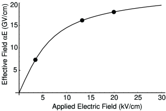
Figure 1: Enhancement factor for YbF. The dots indicate field values at which we have recorded EDM data.

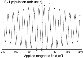
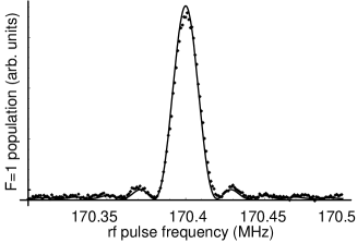
[htb]   a) YbF interferometer fringes. Dots: $F=1$ population measured by fluorescence. Curve: Calculated fringes with normalisation and magnetic field offset as free parameters. Variation of fringe visibility is due to the known beam velocity distribution. b) Lineshape for rf beam splitter. Dots: experiment. Line: model with 50$\mu$s rf pulse length.

Our experiment uses a cold, pulsed, supersonic beam of YbF radicals Tarbutt in a magnetically shielded vertical vacuum chamber $\sim 1.5$m high. The electronic, rotational and vibrational ground state $X^{2}\Sigma^{+}_{1/2},N=0,v=0$ is a hyperfine doublet with states $F=0,1$ split by 170 MHz. We first deplete the $F=1$ state by laser excitation of the $F=1$ molecules on the $A_{1/2}\leftarrow X$ transition. This laser beam is called the pump. A radiofrequency magnetic field, which we call the first beam splitter, then drives the $F=0$ molecules into a symmetric coherent superposition of the $F=1,m_{F}=\pm 1$ states, as described later in more detail. Next, parallel dc electric and magnetic fields are applied to introduce a phase shift $\Delta\phi=\frac{2}{\hbar}\int_{0}^{\tau}(d_{e}\ \alpha(E)\ E(t)+\mu\ \beta(B)\ B(t))\mathrm{d}t$ between the two superposed states. Here $E$ and $B$ appear as functions of time because they are the fields in the molecular rest frame. At time $\tau$ the molecules interact with a second oscillating field, the recombining beam-splitter, that couples the symmetric part of the $F=1$ coherence back to the $F=0$ state. The resulting $F=0$ state population exhibits the usual $\cos^{2}\left(\Delta\phi/2\right)$ fringes of an interferometer. We detect the complementary $F=1$ population using fluorescence induced by a probe laser on the $A_{1/2}\leftarrow X$ transition. Figure 1 shows the interference fringes observed in this fluorescence when the magnetic field is scanned.

The beam splitter is an rf magnetic field perpendicular to $\bf{E}$ and along the beam direction. When a pulse of molecules arrives at the centre of the rf loop it is subject to a short pulse of resonant $170\,$MHz radiation, which induces hyperfine population transfer. It is important that the molecules move as little as possible during this transition because unwanted phase shifts can occur if the fields $E(t)$ or $B(t)$ rotate during the splitting (or recombining) transition. When combined with other imperfections of the apparatus, such a phase can produce a false EDM and is therefore undesirable. Figure 1 shows the lineshape measured using a $50\,\mu$s-long rf pulse, together with a fit to the standard Rabi formulaicols showing good agreement. With high power amplifiers, we are now able work with pulses $10\,\mu$s long, corresponding to a beam movement below 6 mm. The peak transition probability in Figure 1, taken using the first loop, is approximately 0.8. This is due to the beam velocity spread, which gives the gas pulse a length of 5 cm at the first loop and 10 cm at the second. Since the rf field strength varies along the beam line, this spatial spread produces a small distribution of Rabi frequencies, which could be improved by having a more monoenergetic beam.

The arrival of each YbF pulse at our detector is recorded with $1\mu\textrm{s}$ resolution. This time-resolved data gives us a spatial resolution of $\sim 5\ \textrm{mm}$ at the second rf loop. This is the basis of a useful diagnostic technique: varying the timing of the rf pulse allows us to map out the field distribution in the apparatus. This works very well for electric fields because the Stark shift of the hyperfine transition is large. It can also be used to probe magnetic fields, albeit with slightly lower spatial resolution.

3 Noise and systematic effects

With the YbF interferometer working as described above, the electron EDM measurement is straightforward in principle. A small magnetic field is applied to bias the interferometer phase to the point of highest slope. The applied electric field is then reversed and the change in the interferometer output constitutes the EDM signal. In practice, we also reverse the direction of the magnetic field and modulate its amplitude. The EDM is correlated with the relative direction of E and B while the signals demodulated on the individual switching channels yield valuable information about the drift of the interferometer setup and some systematic effects. Additional modulations can be applied: the relative phase between the splitter and recombiner rf fields, the laser frequency, the rf amplitudes and the rf frequencies.

[b]   a) Measured noise power spectrum. Solid line: $1/f$ noise, Dashed line: expected shot noise level. b) Distribution of some 9500 individual EDM measurements, each normalised to its own standard deviation. The solid curve is a Gaussian of unit width. There are clearly excess points in the wings, producing a corresponding deficit at the centre. These are due to the non-statistical behaviour of the noise.

With four switching channels (e.g. E reversal, B reversal, relative rf phase and a small step $\Delta B$) there are sixteen possible states of the machine. We cycle through all of them 256 times to form a “block” of data consisting of 4096 individual points. The repetition rate is determined by the 25Hz ablation laser which forms the YbF beam, thus each block of data requires about $3\,$minutes of real time to record. Slow drifts in the signal are cancelled by choosing appropriate modulation waveforms for the switching channels harrison . Figure 3 shows the power spectrum of the noise in our molecular beam signal, as measured by the photomultiplier recording laser-induced fluorescence from the $F=1$ state. Above about 10Hz the spectrum is largely flat, as one would expect for shot noise due to the statistics of the photon arrivals, but at lower frequencies $1/f$ noise dominates. For this reason, the noise we observe in our EDM measurement usually exceeds the shot noise level. When the ablation target is moved to expose a fresh spot to the YAG laser the excess is typically a factor of 1.5, increasing to 2 over the course of an hour or so, at which point we reset the target.

This non-statistical contribution to the noise in the EDM measurement generates excess noise in the wings of the normalized distribution shown in figure 3. Although it is a small effect, this must be taken into account if we are to assign reliable confidence limits to our EDM measurement. We use a novel bootstrap method. The basic idea is that the experiment itself provides the best available estimate of the true underlying probability distribution bootstrap . Each block of data provides a measurement of the EDM. By randomly choosing values of the EDM from this experimental data set, we create an ensemble of additional synthetic EDM data sets having the same distribution. Note that chosen points are not removed from the pool. Statistical averages are then performed using these empirical data sets. This method works without needing any analytic model for the probability distribution; in particular, we avoid making the usual assumption of a normal distribution. Figure 3 shows the bootstrapped sampling distribution for our 13kV/cm data set and the corresponding cumulative distribution. One sees that the bootstrap method is putting excess probability into the wings of the distribution, as expected. The integral of this probability distribution tells us that the true confidence limits are about 20% larger than one would derive from applying normal Gaussian statistics to the data set.

[t]   The bootstrap analysis. a) Bootstrapped EDM probability distribution around the mean. The solid curve is a normal distribution. b) Cumulative probability, integrating up from below the mean for normal (dashed) and bootstrapped (solid) statistics.

The fluctuating magnetic field in the laboratory is a possible source of additional noise in the measured EDM (or worse, a systematic error if changes in the laboratory field are correlated with the switching of the electric field). The YbF beam is protected from external fields by two layers of magnetic shielding; a flux gate magnetometer between the shields monitors the residual field during data collection. Figure 3 shows the correlation between the field measured by the molecular beam and by the magnetometer, both multiplied by $\mu_{B}/(\alpha E)$ to express them in units of EDM. The slope of the line shows that the shielding factor of the inner shield is approximately $100$. As there is no correlation between the external B field and the electric field reversal, we are confident that this magnetic field noise does not generate a false EDM at the present level of sensitivity.

We employ a veto which discards data when the external field noise exceeds a certain threshold. This improves the uncertainty in the EDM measurement, as illustrated in figure 3 for a subset of our data. This plots the 67% confidence limit on the EDM vs. the magnetic field veto level. The optimal cutoff level is approximately where the external magnetic field induces fluctuations comparable to the EDM measurement error bar. A veto at this level typically rejects about 15% of our data.

[t]   Magnetic noise. a) Correlation between the magnetic field measured by molecules vs. field monitored externally. b) EDM confidence limits as a function of magnetic veto for normal and bootstrapped statistics. The dashed line shows the analysis veto level.

During EDM data acquisition runs, we periodically reverse the electric and magnetic connections to the apparatus manually. This guards against a false EDM generated by the external apparatus (for example magnetic fields from the high voltage relays) or the data acquisition electronics. Because the experiment has been carefully designed to minimize such effects, we do not find any signal correlated with these manual reversals. The saturation of the enhancement shown in figure 1 is another powerful discriminant against systematics. The interferometer phase induced by a true EDM would have to vary in this way, whereas a systematic error would be unlikely to do so. For example, the phase shift due to the magnetic field of a relay is constant, whilst the effect of leakage currents or electrical breakdown grows linearly or faster with the applied voltage. We have recorded data at the field values indicated in the figure. From the data taken so far, we can already see that we do not have any strong disagreement with the result of reference Commins02 , however we have discovered a new systematic effect that needs to be addressed before we can confidently give a new result at a higher level of accuracy.

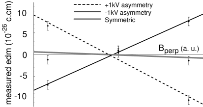
Figure 2: False EDM due to asymmetric field rotation in a perpendicular magnetic field.

As noted previously, the tensor Stark splitting causes the Zeeman shift to depend only on the magnetic field component $B_{z}$ along the electric field direction. As a result, false EDMs due to the $\textrm{v}\times E$ motional field and to geometric phases induced by rotating magnetic fields are utterly negligible for the current beam experiment. This strong coupling of the molecular axis to the external electric field is a major blessing, however, it does also bring with it a potential problem. If the direction of the electric field does not reverse exactly when the voltages are switched, this change of z-axis can produce a change of $B_{z}$ and hence a Zeeman shift that mimics an EDM. In our apparatus, the electric field plates are split into three regions so that the splitter and recombiner transitions can take place at a lower field than the central field region of the interferometer. In the gaps between these regions, the field lines are curved, causing off-axis molecules to experience a rotation of the local z-axis as they fly through. If the electric field were to reverse perfectly this would not cause a problem since the rotation angle would be the same for both electric polarities, but of course no reversal can be perfect. Consequently, a fixed magnetic field roughly perpendicular to the rotating electric field can induce a false EDM. We have demonstrated this by applying a strong perpendicular magnetic field and deliberately introducing a very large asymmetry when the electric field reverses. Figure 2 shows a large false EDM induced in this way. Under our normal operating conditions, we estimate that this effect should not be larger than $\sim 10^{-28}\ \textrm{e.cm}$.

Because it is difficult to guarantee that we understand these fringe fields perfectly and because we are aiming to measure $d_{e}$ at the $\sim 10^{-28}\ \textrm{e.cm}$ level of accuracy, we are now replacing the electrode structure with a single pair of field plates so that the molecules will experience the same magnitude and direction of electric field throughout the entire interferometer. In the new high-field splitter and recombiner regions, the field must be homogeneous across the beam to within 0.1% in order to avoid excessive Stark broadening of the rf transition. This places severe limits on the parallelism of the plates but the required precision has been achieved with specialist machining techniques and the new plates are being installed at time of writing.

4 Outlook

At present we anticipate making a measurement with accuracy in the $10^{-28}\textrm{e.cm}$ range as soon as the new plates are working, which will improve on the result of ref. Commins02 . Over the next few years we expect to reach an accuracy of $1\times 10^{-28}\textrm{e.cm}$ without additional major modifications. In order to be sure of systematics at this level, it may also be necessary to perform a control experiment using CaF molecules. These are similar to YbF structurally and magnetically, but have $\sim 40$ times less sensitivity to the electron EDM according to the expected $Z^{3}$ scaling physica_scripta . We have already made a cold supersonic CaF beam in our apparatus and have seen the transitions that are needed.

It seems possible to go significantly further in measurement accuracy by decelerating the YbF molecules to increase the time that they spend in the interferometer. With this in mind, we have demonstrated that our YbF beam can be decelerated decelerator and we have made substantial progress in understanding how to bring heavy polar molecules close to rest using an alternating gradient decelerator AG review . With the use of an intense, slow YbF beam, there is no obvious obstacle to a measurement at the level of $1\times 10^{-29}\textrm{e.cm}$. Such high precision would provide a probe of new CP-violating elementary particle physics up to mass scales in the range of many TeV, testing some models far beyond the reach of current accelerators including the LHC at CERN.

References

- (1) B.C. Regan et al., Phys. Rev. Lett. 88, 071805 (2002).
- (2) E. N. Fortson, P. Sandars, and S. Barr, Phys. Today 56, No. 6, 33 (2003).
- (3) I.B. Khriplovich and S.K. Lamoreaux, CP violation without strangeness. (Springer, Berlin 1997); Maxim Pospelov and Adam Ritz, Annals Phys. 318, 119-169 (2005).
- (4) A.D. Sakharov, Pis’ma ZhETF 5, 32 (1967). [Sov. Phys. JETP Lett. 5, 24 (1967)]; M Dine, A Kusenko, Rev. Mod. Phys. 76, 1 (2004).
- (5) P.G.H. Sandars, Phys. Lett. 14, 194 (1965).
- (6) Z.W. Liu and H. P. Kelly, Phys. Rev. A 45, R4210 (1992).
- (7) Karin Sangster et al., Phys. Rev. Lett. 71, 3641 (1993); Phys. Rev. A. 51, 1776 (1995).
- (8) E. A. Hinds, Physica Scripta T70, 34 (1997).
- (9) P.G.H. Sandars in Atomic Physics 4 ed. G. zu Putlitz, (Plenum, 1975) p.71.
- (10) M.G. Kozlov and V.F. Ezhov, Phys. Rev. A49, 4502 (1994); M.G. Kozlov, J. Phys. B 30 L607 (1997); A. V. Titov, N. S. Mosyagin, V. F. Ezhov, Phys. Rev. Lett. 77 5346 (1996); H.M. Quiney, H. Skaane, I.P. Grant, J. Phys. B 31 L85 (1998)(after correcting for the trivial factor of 2 between s and their result becomes 26 GV/cm); F.A. Parpia, J. Phys. B 31 1409 (1998); N. Mosyagin, M. Kozlov, A. Titov, J. Phys. B 31 L763 (1998).
- (11) J. J. Hudson et al., Phys. Rev. Lett. 89, 023003 (2002).
- (12) M. R. Tarbutt et al., J. Phys. B 35, 5013 (2002).
- (13) J. J. Hudson, P. C. Condylis, H. T. Ashworth, M. R. Tarbutt, B. E. Sauer and E. A Hinds, in Proceedings of the 17th Conference on Laser Spectroscopy (World Scientific, Singapore 2005), p.129-136
- (14) Norman F. Ramsey, Molecular beams, (Oxford University Press, 1956).
- (15) P. C. Condylis et al., J. Chem. Phys. 123 231101 (2005).
- (16) G. E. Harrison, M. A. Player, and P. G. H. Sandars, J. Phys. E 4, 750 (1971).
- (17) B. Efron and R. Tibshirani, Stat. Sci. 1, 54 (1986).
- (18) M.R. Tarbutt et al., Phys. Rev. Lett., 92, 173002 (2004).
- (19) H. L. Bethlem et al., J. Phys. B., 39, R263-R291 (2006).