Networks of companies and branches in Poland

1 Introduction

During the last few years various models of networks przegl1 ; przegl2 have become a powerful tool for analysis of complex systems in such distant fields as Internet net1 , biology bio1 , social groups social1 , ecology eco1 and public transport julian1 . Modeling behavior of economical agents is a challenging issue that has also been studied from a network point of view. The examples of such studies are models of financial networks CBG , supply chains HL ; HL2 , production networks WB , investment networks BZ or collective bank bankrupcies agata1 ; agata2 . Relations between different companies have been already analyzed using several methods: as networks of shareholders GSB , networks of correlations between stock prices stock1 or networks of board directors board . In several cases scaling laws for network characteristics have been observed.

In the present study we consider relations between companies in Poland taking into account common branches they belong to. It is clear that companies belonging to the same branch compete for similar customers, so the market induces correlations between them. On the other hand two branches can be related by companies acting in both of them. To remove weak, accidental links we shall use a concept of threshold filtering for weighted networks where a link weight corresponds to a number of existing connections (common companies or branches) between a pair of nodes.

2 Bipartite graph of companies and trades

We have used the commercial database ”Baza Kompass Polskie Firmy B2B” from September 2005. It contains information about over 50 000 large and medium size Polish companies belonging to one or more of 2150 different branches. We have constructed a bipartite graph of companies and trades in Poland as at Fig. 1.

Figure 1: Bipartite graph of companies and trades.

In the bipartite graph we have two kinds of objects: branches $A=1,2,3....N_{b}$ and companies $i=1,2,3......N_{f}$, where $N_{b}$ – total number of branches and $N_{f}$ – total number of companies. Let us define a branch capacity $|Z(A)|$ as the cardinality of set of companies belonging to the branch $A$. At Fig. 1 the branch $A$ has the capacity $|Z(A)|=2$ while $|Z(B)|=3$ and $|Z(C)|=1$. The largest capacity of a branch in our database was $2486$ (construction executives), the second largest was $2334$ (building materials).

Let $B(i)$ be a set of branches a given company $i$ belongs to. We define a company diversity as $|B(i)|$. An average company diversity $\mu$ is given as

$$\mu=\frac{1}{N_{f}}\sum^{i=N_{f}}_{i=1}|B(i)|$$ (1)

For our data set we have $\mu=5.99$.
Similarly an average branch capacity $\nu$ is given as

$$\nu=\frac{1}{N_{b}}\sum^{A=N_{b}}_{A=1}|Z(A)|$$ (2)

and we have $\nu=134$.
It is obvious that the following relation is fulfilled for our bipartite graph:

$$\frac{\nu}{N_{f}}=\frac{\mu}{N_{b}}.$$ (3)

3 Companies and trades networks

The bipartite graph from Fig. 1 has been transformed to create a companies network, where nodes are companies and a link means that two connected companies belong to at least one common branch. If we used the example from Fig.1 we would obtain a companies network presented at Fig. 2.

Figure 2: Companies network.

We have excluded from our dataset all items that correspond to communities (local administration) and for our analysis we consider $N_{f}=48158$ companies. All companies belong to a single cluster. Similarly a trade (branch) network has been constructed where nodes are trades and an edge represents connection if at least one company belongs to both branches. In our database we have $N_{b}=2150$ different branches.

Figure 3: Trades network.

4 Weight, weight distribution and networks with cutoffs

We have considered link-weighted networks. In the branches network the link weight means a number of companies that are active in the same pair of branches and it is formally a cardinality of a common part of sets $Z(A)$ and $Z(B)$, where $Z(A)$ is a set of companies belonging to the branch $A$ and $Z(B)$ is a set of companies belonging to the branch $B$.

$$w_{AB}=|Z(A)\cap Z(B)|$$ (4)

Let us define a function $f_{k}^{A}$ which is equal to one if a company $k$ belongs to the branch $A$, otherwise it is zero.

$$f_{k}^{A}=\left\{\begin{array}[]{l}1,k\in A\\ 0,k\notin A\end{array}\right\}$$ (5)

Using the function $f_{k}^{A}$ the weight can be written as:

$$w_{AB}=\sum_{k=1}^{N_{F}}f_{k}^{A}f_{k}^{B}$$ (6)

The weight distribution $p(w)$, meaning the probability $p$ to find a link with a given weight $w$, is presented at Figure 4. The distribution is well approximated by a power function

$$p(w)\sim w^{-\gamma}$$ (7)

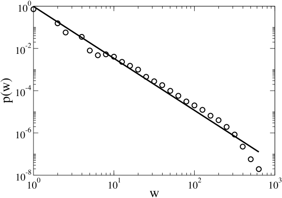
Figure 4: Weight distribution in branches network.

where the exponent $\gamma=2.46\pm 0.07$. One can notice the existence of edges with large weights. The maximum weight value is $w_{max}=764$, and the average weight

$$\langle w\rangle=\sum^{w_{max}}_{w_{min}}wp(w)$$ (8)

equals $\langle w\rangle=4.67$.

Using cutoffs for link weights we have constructed networks with different levels of filtering. In such networks nodes are connected only when their edge weight is no less than an assumed cutoff parameter $w_{o}$.

Table 1: Data for branches networks: $w_{o}$ is the value of selected weight cutoff, $N$ is the number of vertex with nonzero degrees, $E$ is the number of links, $k_{max}$ is the maximum node degree, $\langle k\rangle$ is the average node degree, $C$ is the clustering coefficient.

$w_{o}$	$N$	$E$	$k_{max}$	$\langle k\rangle$	$C$
1	2150	389542	1716	362	0.530
2	2109	212055	1381	201	0.565
3	2053	136036	1127	132	0.568
4	2007	100917	952	100	0.575
5	1948	80358	802	82	0.589
1	2150	389542	1716	362	0.530
2	2109	212055	1381	201	0.565
3	2053	136036	1127	132.	0.568
4	2007	100917	952	100	0.575
5	1948	80358	802	82	0.589
6	1904	66353	655	69	0.592
7	1858	56565	569	60	0.596
8	1819	49193	519	54	0.597
9	1786	43469	477	48	0.599
10	1748	38924	450	44	0.600
12	1666	32167	394	38	0.615
14	1611	26088	325	32	0.605
16	1545	21762	288	28	0.606
18	1490	18451	259	24	0.603
20	1424	15872	226	22	0.604
30	1188	8989	162	15	0.585
40	996	6036	131	12	0.587
50	857	4379	111	10	0.572
60	752	3303	85	8	0.551
70	666	2638	65	7	0.524
80	575	2143	55	7	0.532
90	512	1808	49	7	0.538
100	464	1543	41	6	0.546
150	306	750	26	4	0.493

A weight in the companies network is defined in a similar way as in the branches networks, i.e. it is the number of common branches for two companies — formally it is equal to the cardinality of a common part of sets $B(i)$ and $B(j)$, where $B(i)$ is a set of branches the company $i$ belongs to, $B(j)$ is a set of branches the company $j$ belongs to.

$$w_{ij}=|B(i)\cap B(j)|$$ (9)

Using the function $f_{k}^{A}$ the weight can be written as

$$w_{ij}=\sum_{A=1}^{N_{b}}f_{i}^{A}f_{j}^{A}.$$ (10)

The maximum value of observed weights $w_{max}=207$ is smaller in this networks than in the branches network while the average value equals $\langle w\rangle=1.48$. The weight distribution is not a power law in this case and it shows an exponential behavior in a certain range.

Similarly to the branches networks we have introduced cutoffs in companies network. At the Fig.5 we present average degrees of nodes and maximum degrees as functions of the cutoff parameter $w_{o}$.

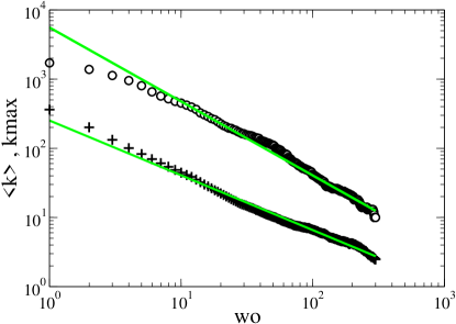
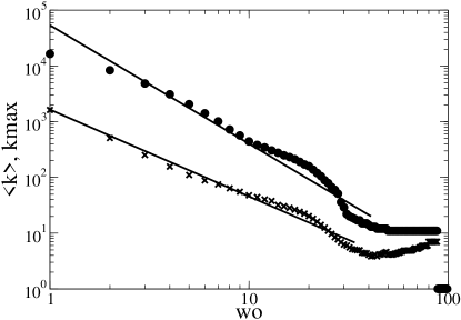
Figure 5: Dependence of $\langle k\rangle$ and $k_{max}$ on cutoff parameter $w_{o}$ for branches networks (left) and companies networks (right).

We have observed a power law scaling

$$\langle k\rangle\sim w_{o}^{-\beta}$$ (11)

$$k_{max}\sim w_{o}^{-\alpha}$$ (12)

where for branches networks $\alpha_{b}=1.069\pm 0.008$ and $\beta_{b}=0.792\pm 0.005$ while for companies networks $\alpha_{f}=2.13\pm 0.07$ and $\beta_{f}=1.55\pm 0.04$.

Table 2: Data for companies networks: $w_{o}$ is the selected cutoff, $N$ is the number of nodes with nonzero degrees, $E$ is the number of links, $k_{max}$ is the maximum node degree, $\langle k\rangle$ is the average node degree, $C$ is the clustering coefficient.

$w_{o}$	$N$	$E$	$k_{max}$	$\langle k\rangle$	$C$
1	48158	39073685	16448	1622	0.652
2	39077	9932790	8366	508	0.689
3	31150	3928954	4842	252	0.714
4	24212	1895373	3103	156	0.717
5	18566	1024448	2059	110	0.713
6	14116	622662	1412	88	0.710
7	10796	404844	1012	74	0.700
8	8347	266013	724	63	0.701
9	6527	180696	566	55	0.699
10	5197	124079	443	47	0.699
11	4268	94531	382	44	0.704
12	3400	68648	345	40	0.693
13	2866	54258	305	37	0.691
14	2277	36461	277	32	0.663
15	1903	28844	249	30	0.673
16	1627	23063	231	28	0.678
17	1397	18352	212	26	0.667
18	1196	14480	191	24	0.680
19	1003	11230	171	22	0.680
20	883	8907	159	20	0.676

5 Degree distribution

We have analyzed the degree distribution for networks with different cutoff parameters. At Fig. 6 we present the degree distributions for companies networks for different values of $w_{o}$. The distributions change qualitatively with increasing $w_{o}$ from a nonmonotonic function with an exponential tail (for $w_{o}=1$) to a power law with exponent $\gamma$ (for $w_{o}>6$).

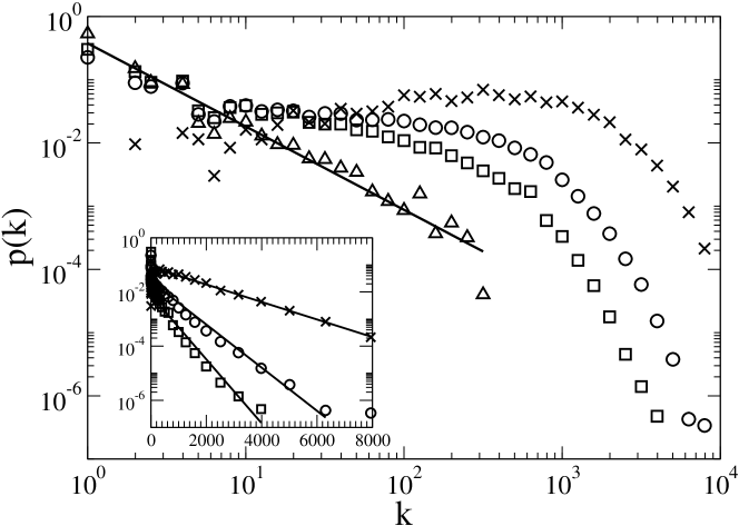
Figure 6: Degree distributions for companies networks for different values of $w_{o}$. X-marks are for $w_{o}=1$, circles are for $w_{o}=2$, squares are for $w_{o}=3$ and triangles are for $w_{o}=12$.

Values of exponent $\gamma$ for different cutoffs are given in the Table 3.

Table 3: Values of exponent $\gamma$ for different cutoffs $w_{o}$ in companies networks.

$w_{o}$	$\gamma$	$\Delta\gamma$
6	1.06	0.03
8	1.12	0.04
10	1.22	0.05
12	1.23	0.06
14	1.31	0.05
16	1.31	0.06
18	1.37	0.07
20	1.35	0.07

Now let us come back to branches networks. At the Fig. 7 we present a degree distribution for $w_{o}=1$. We observe a high diversity of node degrees — vertices with large values of $k$ occur almost as frequent as vertices with a small $k$.

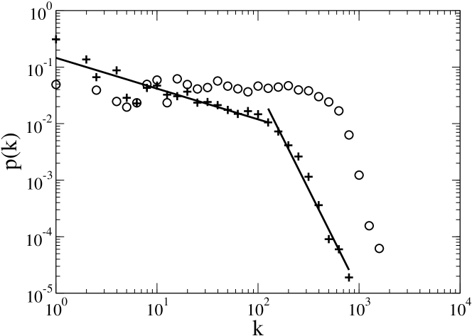
Figure 7: Degree distribution in branches network for different values of $w_{o}$. Circles are for $w_{o}=1$, crosses are for $w_{o}=4$.

For a properly chosen cutoff values the degree distributions are described by power laws. For $w_{o}=4$ we see two regions of scaling with different exponents $\gamma_{1}$ and $\gamma_{2}$ while a transition point between both scaling regimes appears at $k\approx 100$. The transition appears due to the fact that there are almost no companies with diversity over $100$, so branches with $k>100$ have connections due to several companies, as opposed to branches with $k<100$ that can be connected due to a single company. However the probability that many companies link a single branch with many different others is low, thus the degree probability $p(k)$ decays much faster after the transition point. In the Table 4 we present values $\gamma_{1}$ and $\gamma_{2}$ for different cutoffs $w_{o}$.

Table 4: Values of scaling exponents $\gamma_{1}$ and $\gamma_{2}$ for branches networks.

$w_{o}$	$\gamma_{1}$	$\Delta\gamma_{1}$	$\gamma_{2}$	$\Delta\gamma_{2}$
4	0.54	0.06	3.56	0.22
5	0.59	0.05	3.70	0.21
6	0.62	0.06	3.60	0.22
7	0.64	0.07	3.44	0.19
8	0.69	0.06	3.53	0.22
9	0.72	0.06	3.67	0.26
10	0.75	0.06	3.68	0.21
12	0.80	0.06	3.98	0.38
14	0.83	0.07	3.63	0.27
16	0.86	0.0	3.52	0.26
18	0.89	0.11	3.39	0.12
20	0.93	0.07	3.52	0.20
30	1.15	0.08	3.66	0.44
40	1.21	0.09	3.43	0.31
50	1.28	0.10	3.51	0.39
60	1.39	0.11	3.77	0.67
70	1.47	0.11	4.07	0.69

It is important to stress that in both networks (companies and branches) the scaling behavior for degree distribution occurs only if we use cutoffs for links weights, compare Fig. 6 and Fig. 7. It follows that such cutoffs act as filters for the noise present in the complex network topology.

6 Entropy of network topology

Having a probability distribution of node degrees one can calculated a corresponding measure of network heterogeneity. We have used the standard formula for Gibbs entropy, i.e.

$$S=-\sum_{k}p(k)\ln p(k)$$ (13)

The entropy of degree distribution in branches networks decays logarithmically as a function of the cutoff value (Fig. 8)

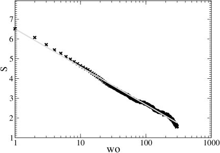
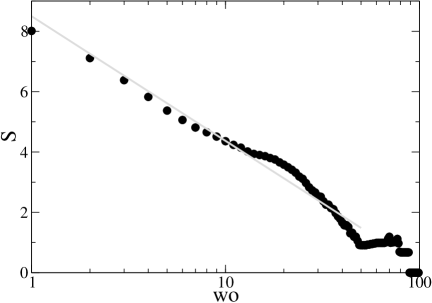
Figure 8: Entropy dependence on cutoff parameter for branches networks on the left and for companies networks on the right.

$$S=-a\ln(w_{o})+b$$ (14)

where $a=0.834\pm 0.004$ and $b=6.51\pm 0.02$. The entropy in companies networks behaves similarly with $a=1.79\pm 0.05$ and $b=8.49\pm 0.15$.

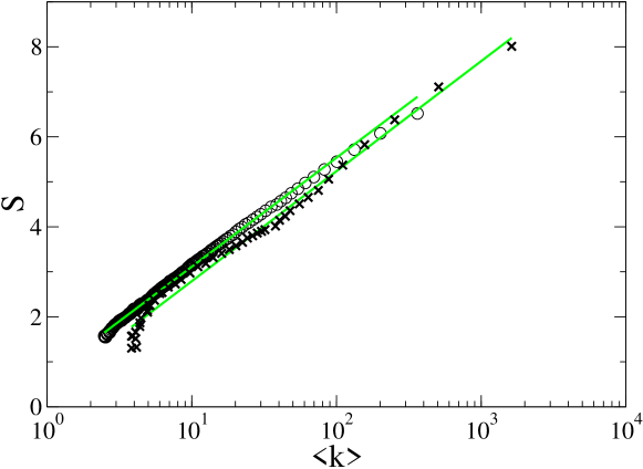
Figure 9: Dependence of entropy on the average nodes degree. Circles represent branches networks and X-marks represent companies networks.

The behavior has the following explanation. Diversity of node degrees is decreasing with growing weight cutoff values $w_{o}$. Larger cutoffs reduce total number of links in the network what leads to a smaller range of $k$ and thus to smaller values of $k_{max}$ and $\langle k\rangle$. The relation between $S$ and $\langle k\rangle$ is presented at the Fig. 9, where a logarithmic scaling can be seen

$$S\sim\alpha\ln\langle k\rangle$$ (15)

with $\alpha=1.052\pm 0.003$ for branches networks and $\alpha=1.062\pm 0.019$ for companies networks.

7 Clustering coefficient

We have analyzed a clustering coefficient dependence on node degree in branches and companies networks.

Figure 10: Clustering coefficient dependence on node degree for $w_{o}=1$. Circles are for companies network and squares are for branch networks.

In the companies network the clustering coefficient for small values of $k$ is close to one, for larger $k$ the value of $C(k)$ exhibits logarithmic behavior

$$C\sim\beta\ln k$$ (16)

with $\beta_{1}=-0.174\pm 0.006$. In branches networks the logarithmic behavior is present for the whole range of $k$ with $\beta_{2}=-0.111\pm 0.004$.

8 Conclusions

In this study, we have collected and analyzed data on companies in Poland. $48158$ medium/large firms and $2150$ branches form a bipartite graph that allows to construct weighted networks of companies and branches.

Link weights in both networks are very heterogenous and a corresponding link weight distribution in the branches network follows a power law. Removing links with weights smaller than a cutoff (threshold) $w_{o}$ acts as a kind of filtering for network topology. This results in recovery of a hidden scaling relations present in the network. The degree distribution for companies networks changes with increasing $w_{o}$ from a nonmonotonic function with an exponential tail (for $w_{o}=1$) to a power law (for $w_{o}>6$). For a filtered ($w_{o}>4$) branches network we see two regions of scaling with different exponents and a transition point between both regimes. Entropies of degree distributions of both networks decay logarithmically as a function of cutoff parameter and are proportional to the logarithm of the mean node degree.

9 Acknowledgements

We acknowledge a support from the EU Grant Measuring and Modeling Complex Networks Across Domains — MMCOMNET (Grant No. FP6-2003-NEST-Path-012999) and from Polish Ministry of Education and Science (Grant No. 13/6.PR UE/2005/7).

References

- (1) Albert R, Barabasi A-L (2002) Statistical mechanics of complex networks, Reviews of Modern Physics 74:47-97
- (2) Newman M E J (2003) The structure and function of complex networks, SIAM Review 45:167-256
- (3) Pastor-Satorras P, Vespignani A (2004) Evolution and structure of the internet: a statistical physics approach, Cambridge University Press, Cambridge
- (4) Ravasz E, Somera AL, Mongru DA, Oltvai ZN, Barabasi A-L (2002) Hierarchical organization of modularity in metabolic networks, Science 297:1551-1555
- (5) Newman MEJ, Park J (2003) Why social networks are different from other types of networks, Physical Review E 68:036122
- (6) Garlaschelli D, Caldarelli G, Pietronero L (2003) Universal scaling relations in food webs, Nature 423:165-168
- (7) Sienkiewicz J, Holyst JA (2005) Statistical analysis of 22 public transport networks in Poland, Physical Review E, 72:046127
- (8) Caldarelli G, Battiston S, Garlaschelli D, Catanzaro M (2004) Emergence of Complexity in Financial Networks. In: Ben-Naim E, Frauenfelder H, Toroczkai Z (eds) Lecture Notes in Physics 650:399 - 423, Springer-Verlag
- (9) Helbing D, Lammer S, Seidel T (2004) Physics, stability and dynamics of supply newtoks, Physical Review E 70:066116
- (10) Halbing D, Lammer S, Witt U, Brenner T (2004) Network-induced oscillatory behavior in material flow networks and irregular business cycles, Physical Review E, 70:056118
- (11) Weisbuch G, Battiston S (2005) Production networks and failure avalanches e-print physics/0507101
- (12) Battiston S, Rodrigues JF, Zeytinoglu H (2005) The Network of Inter-Regional Direct Investment Stocks across Europe e-print physics/0508206
- (13) Aleksiejuk A, Holyst JA (2001) A simple model of bank bankruptcies, Physica A, 299:198-204
- (14) Aleksiejuk A, Holyst JA, Kossinets G (2002) Self-organized criticality in a model of collective bank bankruptcies, International Journal of Modern Physics C, 13:333-341
- (15) Garlaschelli G, Battiston S (2005) The scale-free topology of market investments, Physica A, 350:491-499
- (16) Onella J-P, Chakraborti A, Kaski K, Kertesz J, Kanto A (2003) Dynamics of market correlations: Taxonomy and portfolio analysis, Physical Review E, 68:056110
- (17) Battiston S, Catanzaro M (2004) Statistical properties of corporate board and director networks, European Physical Journal B 38:345-352