Bound state equivalent potentials with the Lagrange mesh method

Abstract

The Lagrange mesh method is a very simple procedure to accurately solve eigenvalue problems starting from a given nonrelativistic or semirelativistic two-body Hamiltonian with local or nonlocal potential. We show in this work that it can be applied to solve the inverse problem, namely, to find the equivalent local potential starting from a particular bound state wave function and the corresponding energy. In order to check the method, we apply it to several cases which are analytically solvable: the nonrelativistic harmonic oscillator and Coulomb potential, the nonlocal Yamaguchi potential and the semirelativistic harmonic oscillator. The potential is accurately computed in each case. In particular, our procedure deals efficiently with both nonrelativistic and semirelativistic kinematics.

I Introduction

The Lagrange mesh method is a very accurate and simple procedure to compute eigenvalues and eigenfunctions of a two-body Schrödinger equation baye86 ; vinc93 ; baye95 . It is applicable for both local and nonlocal interactions nonloc , and also for a semirelativistic kinetic operator, i.e. the spinless Salpeter equation sem01 ; brau2 . In this method, the trial eigenstates are developed in a basis of well-chosen functions, the Lagrange functions, and the Hamiltonian matrix elements are obtained with a Gauss quadrature. Moreover, the Lagrange mesh method can be extended to treat very accurately three-body problems, in nuclear or atomic physics hess99 ; 3b2 .

In this work, we apply the Lagrange mesh method to solve the inverse problem for bound states: starting from a given bound state – wave function and corresponding eigenenergy –, we show how to compute the equivalent local potential. To our knowledge, this application of Lagrange mesh method has not been studied before. It can then be used to compute the equivalent local potential of a given nonlocal potential. The determination of equivalent local potentials is of particular interest in nuclear physics (see for example Ref. nucl ). The more interesting point is that our procedure allows to deal with semirelativistic kinematics.

Our paper is organized as follows. In Sec. II, we recall the main points of the Lagrange mesh method and show how to apply it to solve a bound state problem with a central potential. Then, we give a procedure to compute the equivalent local potential with this method starting from a given spectrum in Sec. III. In order to check the efficiency of our method, we apply it to several cases in which the spectrum is analytically known. Firstly, we consider three central potentials with a nonrelativistic kinematics in Sec. IV: the harmonic oscillator (Sec. IV.1), the Coulomb potential (Sec. IV.2), and the nonlocal Yamaguchi potential (Sec. IV.3). Secondly, in Sec. V, we consider the case of the semirelativistic harmonic oscillator for two massless particles, whose solution is also analytical. The accuracy of the method is checked in all those cases, and conclusions are drawn in Sec. VI.

II Lagrange mesh method

A Lagrange mesh is formed of $N$ mesh points $x_{i}$ associated with an orthonormal set of indefinitely derivable functions $f_{j}(x)$ on an interval $[a,b]$. A Lagrange function $f_{j}(x)$ vanishes at all mesh points but one; it satisfies the condition baye86 ; vinc93 ; baye95

$$f_{j}(x_{i})=\lambda^{-1/2}_{i}\delta_{ij}.$$ (1)

The weights $\lambda_{i}$ are linked to the mesh points $x_{i}$ through a Gauss quadrature formula

$$\int^{b}_{a}g(x)\,dx\approx\sum^{N}_{k=1}\lambda_{k}\,g(x_{k}),$$ (2)

which is used to compute all the integrals over the interval $[a,b]$.

As in this work we only study radial equations, we consider the interval $[0,\infty[$, leading to a Gauss-Laguerre quadrature. The Gauss formula (2) is exact when $g(x)$ is a polynomial of degree $2N-1$ at most, multiplied by $\exp(-x)$. The $N$ Lagrange-Laguerre mesh points $x_{i}$ are then given by the zeros of the Laguerre polynomial $L_{N}(x)$ of degree $N$ baye86 . An explicit form can be derived for the corresponding regularized Lagrange functions

$$f_{i}(x)=(-1)^{i}x^{-1/2}_{i}\,x(x-x_{i})^{-1}L_{N}(x)\,e^{-x/2}.$$ (3)

They clearly satisfy the constraint (1), and they are orthonormal, provided the scalar products are computed with the quadrature (2). Moreover, they vanish in $x=0$.

To show how these elements can be applied to a physical problem, let us consider a standard Hamiltonian $H=T(\vec{p}^{\,2})+V(r)$, where $T(\vec{p}^{\,2})$ is the kinetic term and $V(r)$ a radial potential (we work in natural units $\hbar=c=1$). The calculations are performed with trial states $|\psi\rangle$ given by

$$\left|\psi\right\rangle=\sum^{N}_{k=1}C_{k}\left|f_{k}\right\rangle,$$ (4)

where

$$\left\langle\vec{r}\,|f_{k}\right\rangle=\frac{f_{k}(r/h)}{\sqrt{h}\,r}Y_{\ell m}(\theta,\varphi).$$ (5)

$\ell$ is the orbital angular momentum quantum number and the coefficients $C_{k}$ are linear variational parameters. $h$ is a scale parameter chosen to adjust the size of the mesh to the domain of physical interest. If we define $r=h\,x$, with $x$ a dimensionless variable, a relevant value of $h$ will be obtained thanks to the relation $h=r_{a}/x_{N}$, where $x_{N}$ is the last mesh point and $r_{a}$ is a physical radius for which the asymptotic tail of the wave function is well defined. This radius has to be a priori estimated, but various computations show that it has not to be known with great accuracy, since the method is not variational in $h$ sem01 ; fab1 .

We have now to compute the Hamiltonian matrix elements. Let us begin with the potential term. Using the properties of the Lagrange functions and the Gauss quadrature (2), the potential matrix for a local potential $V(r)$ is diagonal. Its elements are

$$V_{ij}=\int^{\infty}_{0}dx\,f_{i}(x)V(h\,x)f_{j}(x)\approx V(hx_{i})\,\delta_{ij},$$ (6)

and only involve the value of the potential at the mesh points. As the matrix elements are computed only approximately, the variational character of the method cannot be guaranteed. But the accuracy of the method is preserved baye02 . The matrix elements for a nonlocal potential $W(r,r^{\prime})$ are given by nonloc

$$W_{ij}=h\,\int^{\infty}_{0}dx\int^{\infty}_{0}dx^{\prime}f_{i}(x)\,W(hx,hx^{\prime})\,f_{j}(x^{\prime})\approx h\,\sqrt{\lambda_{i}\lambda_{j}}\ W(hx_{i},hx_{j}).$$ (7)

The kinetic energy operator is generally only a function of $\vec{p}^{\,2}$. It is shown in Ref. baye95 that, using the Gauss quadrature and the properties of the Lagrange functions, one obtains the corresponding matrix

$$(\vec{p}^{\,2})_{ij}=\frac{1}{h^{2}}\left[p^{\,2}_{r\,ij}+\frac{\ell(\ell+1)}{x^{2}_{i}}\delta_{ij}\right],$$ (8)

where

$$p^{2}_{r\,ij}=\left\{\begin{array}[]{lll}&(-1)^{i-j}(x_{i}x_{j})^{-1/2}(x_{i}+x_{j})(x_{i}-x_{j})^{-2}&(i\neq j),\\ &(12\,x^{2}_{i})^{-1}[4+(4N+2)\,x_{i}-x^{2}_{i}]&(i=j).\end{array}\right.$$ (9)

Now, the kinetic energy matrix $T(\vec{p}^{\,2})$ can be computed with the following method sem01 :

1. Diagonalization of the matrix $\vec{p}^{\,2}$. If $D^{2}$ is the corresponding diagonal matrix, we have thus $\vec{p}^{\,2}=SD^{2}S^{-1}$, where $S$ is the transformation matrix.

2. Computation of $T(D^{2})$ by taking the function $T$ of all diagonal elements of $D^{2}$.

3. Determination of the matrix elements $T_{ij}$ in the Lagrange basis by using the transformation matrix $S$: $T(\vec{p}^{\,2})=S\,T(D^{2})\,S^{-1}$.

Note that such a calculation is not exact because the number of Lagrange functions is finite. However, it has already given good results in the semirelativistic case, when $T(\vec{p}^{\,2})=\sqrt{\vec{p}^{\,2}+m^{2}}$ sem01 or even when $T(\vec{p}^{\,2},r)=\sqrt{\vec{p}^{\,2}+U^{2}(r)}$ brau2 .

The eigenvalue equation $H\left|\psi\right\rangle=E\left|\psi\right\rangle$ reduces then to a system of $N$ mesh equations,

$$\sum^{N}_{j=1}\left[T_{ij}+{\cal V}_{ij}-E\delta_{ij}\right]C_{j}=0\quad\text{with}\quad C_{j}=\sqrt{h\lambda_{j}}\,u(hx_{j}),$$ (10)

where $u(r)$ is the regularized radial wave function and ${\cal V}$ the local or nonlocal potential matrix. The coefficients $C_{j}$ provide the values of the radial wave function at mesh points. But contrary to some other mesh methods, the wave function is also known everywhere thanks to Eq. (4).

III Bound state equivalent local potential

In the previous section, we applied the Lagrange mesh method to solve the eigenequation for two-body central problems. We now show that this method allows to solve very easily the inverse problem, that is, starting from particular wave function $\left|\psi\right\rangle$ and energy $E$, to find the corresponding equivalent local potential for a given kinematics $T$.

In the case of a local central potential, the mesh equations (10) can be rewritten as

$$V(hx_{i})=E-\frac{1}{\sqrt{\lambda_{i}}\,u(hx_{i})}\sum^{N}_{j=1}T_{ij}\sqrt{\lambda_{j}}\ u(hx_{j}).$$ (11)

We see from the above equation that, provided we know the radial wave function and the energy of the state, the equivalent local potential can be directly computed at the mesh points. Let us note that, since the matrix elements $T_{ij}$ depend on the orbital angular momentum $\ell$, this quantum number has to be a priori specified. The calculation is done easily because the potential matrix for a local potential $V(r)$ is diagonal and only involves the value of the potential at the mesh points, as shown in Eq. (6). Obviously, this method does not require a given normalization for the wave function. Moreover, it is also applicable for semirelativistic kinematics.

We can remark that Eq. (11) contains term which are proportional to $u(hx_{j})/u(hx_{i})$. They may be difficult to compute numerically with a great accuracy when $hx_{i}$ is either close to zero or very large. In these cases indeed, the regularized wave function tends towards zero. It means that the first values of the potential and also the last ones could be inaccurate. It is worth mentioning that, for radially excited states, a particular mesh point $x_{k}$ could be such that $hx_{k}$ is a zero of the wave function. In this case, $V(hx_{k})$ cannot be computed. Although very improbable, this problem could simply be cured by taking a slightly different value of $N$ or $h$.

In order to check the validity of our method, we will consider four cases where the eigenvalue problem is analytically solvable for a given potential $V^{E}$. This will enable us to compare the numerically computed points $V(hx_{i})$ with the corresponding exact values $V^{E}(hx_{i})$. The number $\delta$, defined by

$$\delta=\max\left\{\left|\frac{V(hx_{i})-V^{E}(hx_{i})}{V^{E}(hx_{i})}\right|,\ 3\leq i\leq N-3\right\},$$ (12)

is a measurement of the accuracy of the numerical computations. The more $\delta$ is close to zero, the more the method is accurate. The first and last two mesh points are – arbitrarily – not included in the computation of $\delta$, since they can introduce errors which are not due to the method itself, but rather to a lack of precision in the numerical computations, as we argued previously from inspection of formula (11).

IV Nonrelativistic Applications

The kinetic operator which will be used in all the computations of this section is given by

$$T(\vec{p}^{\,2})=\frac{\vec{p}^{\,2}}{2\mu},$$ (13)

where $\mu$ is the reduced mass of the studied two-body system.

IV.1 Harmonic oscillator

The spectrum of a spherical harmonic oscillator, whose potential reads

$$V^{E}(r)=\frac{\Lambda^{2}r^{2}}{2\mu},$$ (14)

is given by (see for example Ref. (flu, , problem 66))

$$R_{n\ell}(r)\propto r^{\ell}\,{\rm e}^{-\Lambda r^{2}/2}L^{\ell+1/2}_{n}(\Lambda\,r^{2}),\quad E_{n\ell}=\Lambda\,\mu^{-1}(2n+\ell+3/2).$$ (15)

It is readily computed from the virial theorem that $\left\langle r^{2}\right\rangle=(2n+\ell+3/2)/\Lambda$. Therefore, we suggest the following value for the scale parameter:

$$h = \frac{4\sqrt{\left\langle r^{2}\right\rangle}}{x_{N}}$$ (16)

$$= \frac{4}{x_{N}}\sqrt{\frac{(2n+\ell+3/2)}{\Lambda}},$$ (17)

where the factor $4$ ensures that the last mesh point will be located in the asymptotic tail of the wave function.

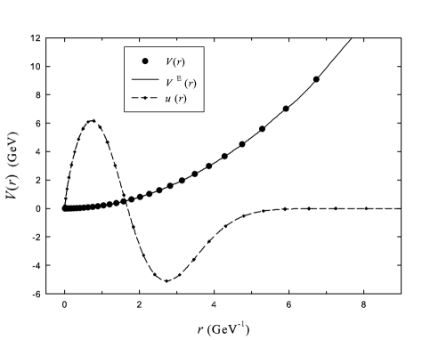
Figure 1: Comparison between the potential computed from the $2S$ wave function (15) thanks to the Lagrange mesh formula (11), and the exact harmonic potential given by Eq. (14). The equivalent potential is only known at the mesh points (circles), and the exact potential is plotted with a solid line. The regularized wave function is also plotted with an arbitrary normalization (dashed line). We used $\mu=0.70$ GeV, $\Lambda=0.53$ GeV ², $N=30$, and $h=9.8~{}10^{-2}$ GeV^-1 following formula (17).

In order to make explicit computations, we have to specify the value of our parameters. We set $\mu=0.70$ GeV and $\Lambda=0.53$ GeV². These parameters can be used in hadron physics to roughly describe a $c\bar{c}$ meson fab1 ; drg . We choose $N=30$, and the scale parameter is computed by using Eq. (17). Once these parameters are fixed, Eqs. (11) and (15) allow to find the equivalent local potential. The result is plotted and compared to the exact harmonic potential (14) in Fig. 1, where we used the wave function in the $2S$ state ($n=1,\,\ell=0$). The numerical result is clearly close to the exact result, and only $30$ mesh points are enough to provide a good picture of the potential: we have indeed $\delta=2.1~{}10^{-3}~{}\%$, this number being computed with Eq. (12). The same conclusion holds if other states than the $2S$ one are used, and $\delta$ is always smaller than $1~{}\%$.

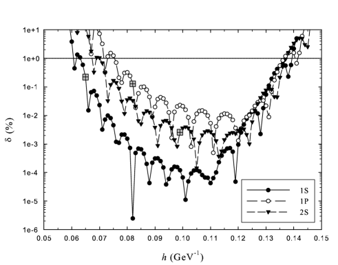
Figure 2: Evolution of $\delta$ versus the scale parameter $h$ for the $1S$ (full circles), $1P$ (empty circles), and $2S$ (triangles) states for $N=30$. The gray boxes are the different values of $\delta$ for a scale parameter computed with formula (17). They all ensure a value of $\delta$ lower than $1~{}\%$.

In Fig. 2, we show the variation of $\delta$ with the scale parameter $h$ for three different states and $N=30$. We can conclude from this figure that a rather large interval exists where the quantity $\delta$ is lower than $1~{}\%$. Consequently, the scale parameter does not need to be computed with great accuracy: our criterion (16) is clearly accurate enough since the predicted value of $h$ is always located in this interval. The global behavior of $\delta$ which can be observed in Fig. 2 is due the difficulty of computing $V(hx_{i})$ when the scale parameter is too small or too large. In this case indeed, the mesh points $hx_{i}$ cover no longer the main part of the wave function, and a partial knowledge of the wave function leads to an inaccurate description of the potential.

IV.2 Coulomb potential

This case is of interest since it enables us to check whether the method we present can correctly reproduce a singular potential or not. The radial wave function and eigenenergies of a central Coulomb potential

$$V^{E}=-\frac{\kappa}{r}$$ (18)

respectively read (see for example Ref. (flu, , problem 67))

$$R(r)\propto r^{\ell}\,{\rm e}^{-\gamma r}\,L^{2\ell+1}_{n_{p}-\ell-1}(2\gamma r),\quad E_{n_{p}}=-\frac{\mu\kappa^{2}}{2n^{2}_{p}},$$ (19)

with $n_{p}\geq 1$, $0\leq\ell\leq n_{p}-1$, and $\gamma=\mu\kappa/n_{p}$. The principal quantum number $n_{p}$ is defined by $n_{p}=n+\ell+1$.

It can be computed that (landau, , p. 147)

$$\left\langle r^{2}\right\rangle=\frac{n^{2}_{p}}{2\mu^{2}\kappa^{2}}\left[5n^{2}_{p}+1-3\ell(\ell+1)\right].$$ (20)

As the evaluation of the scale parameter given by Eq. (16) yields good results in the harmonic oscillator case, it can be adapted to the Coulomb potential, and $h$ is now defined as

$$h=\frac{15}{x_{N}}\frac{n_{p}}{\sqrt{2}\,\mu\kappa}\sqrt{5n^{2}_{p}+1-3\ell(\ell+1)}.$$ (21)

A factor $15$ is now needed because the Coulomb potential is a long- ranged one. The wave function has thus to be known on a larger domain than for the harmonic oscillator, since the latter potential is a confining one.

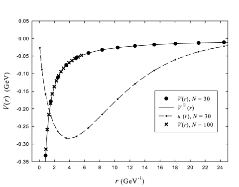
Figure 3: Comparison between the potential computed from the $1S$ wave function (19) thanks to the Lagrange mesh formula (11), and the exact Coulomb potential given by Eq. (18). The potential has been computed with $N=30$ (circles) and $N=100$ (crosses) mesh points, but only a few points are plotted for clarity. The regularized wave function is also plotted with an arbitrary normalization (dashed line). We used $\mu=0.70$ GeV and $\kappa=0.27$. For $N=30$, it can be computed that $h=1.3$ GeV^-1 and $\delta=1.4~{}10^{-5}~{}\%$; for $N=100$, we have $h=0.37$ GeV^-1 and $\delta=0.7~{}\%$.

In order to numerically compute the equivalent potential from the wave function (19), we set $\mu=0.70$ GeV and $\kappa=0.27$. The particular value of $\kappa$ we chose is commonly used in hadron physics to parameterize the one-gluon-exchange part of the potential between two heavy quarks fab1 . We choose $N=30$, and the scale parameter is computed by using Eq. (21). The result is plotted and compared to the exact Coulomb potential (18) in Fig. 3 for the wave function in the ground state ($n=\ell=0$). The numerical result is close to the exact result, with a value of $\delta$ which is equal to $1.4~{}10^{-5}~{}\%$. In particular, the singular behavior is well reproduced. To stress this point, we performed another calculation with $N=100$, and $h=0.37$ GeV^-1 following Eq. (21). It can be seen in Fig. 3 that the Coulomb potential is then very well matched at short distances. In this case however, we have $\delta=0.7~{}\%$. Although this precision is still very satisfactory, it seems strange at first sight that $\delta$ is higher for a larger number of mesh points. This is due to the fact that the mesh points are the zeros of the Laguerre polynomial of degree $N$. The first physical point which is taken into account in the definition of $\delta$ is $hx_{3}$, which is smaller for $N=100$ ($hx_{3}=0.811$ GeV^-1) than for $N=30$ ($hx_{3}=0.068$ GeV^-1). This causes $\delta$ to be larger, since the more a point is close to zero, the more the accuracy decreases.

For what concerns the variation of $\delta$ versus $h$, the same qualitative features than for the harmonic oscillator are observed. Equation (21) thus appears to give a good evaluation of the scale parameter. It can be also checked that a factor smaller than $15$ in Eq. (21) can lead to values of the scale parameter for which $\delta$ is quite larger than $1~{}\%$.

IV.3 Yamaguchi potential

The Yamaguchi potential is a separable nonlocal potential, given by

$$W(r,r^{\prime})=-v(r)\,v(r^{\prime}),$$ (22)

with

$$v(r)=\sqrt{\beta/\mu}\ (\alpha+\beta)\,{\rm e}^{-\beta r}.$$ (23)

It was introduced in Ref. yama to study the deuteron ($\mu=0.468$ GeV). In particular, for $\alpha=0.046$ GeV and $\beta=0.274$ GeV, it admits a bound state whose binding energy is the one of the deuteron, that is $E=-2.225$ MeV.

A nice particularity of this nonlocal potential is that the bound state wave function can be analytically determined. It reads

$$R(r)\propto\frac{{\rm e}^{-\alpha r}-{\rm e}^{-\beta r}}{r}.$$ (24)

Inserting this wave function into Eq. (11) will provide us with the equivalent local potential associated with the Yamaguchi potential. Finding equivalent local potentials coming from nonlocal potentials is of interest in nuclear physics, although most studies are devoted to scattering states (see for example Refs. nucl ). The bound state equivalent potential of a separable nonlocal potential of the form (22) is shown in Ref. dijk to be given by

$$V^{L}(r)=-\frac{v(r)}{u(r)}\int^{\infty}_{0}dr^{\prime}\,v(r^{\prime})\,u(r^{\prime}),$$ (25)

with $u(r)$ the regularized wave function of the bound state for the nonlocal potential. Relations (23) and (24) can be injected in this last equation to compute that

$$V^{L}(r)=-\,\frac{\beta^{2}-\alpha^{2}}{2\mu}\,\frac{{\rm e}^{-\beta r}}{{\rm e}^{-\alpha r}-{\rm e}^{-\beta r}}.$$ (26)

As the radial wave function (24) is maximal in $r=0$, $R(0)\propto(\beta-\alpha)$, we can compute the scale parameter by demanding that

$$R(hx_{N})/R(0)=\epsilon,$$ (27)

with $\epsilon$ a small number, that we will set equal to $10^{-3}$. Then, assuming that $\alpha\ll\beta$ as it is the case for the deuteron, $h$ will approximately be given by

$$h\approx-\frac{\ln\left[\epsilon(\beta-\alpha)\right]}{\alpha\,x_{N}}.$$ (28)

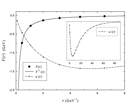
Figure 4: Comparison between the equivalent local potential (circles) computed from the wave function (24) with $E=-2.225$ MeV and the exact equivalent local potential (solid line) given by Eq. (26). The regularized wave function is also plotted with an arbitrary normalization (dashed line). We used $\alpha=0.046$ GeV, $\beta=0.274$ GeV, and $N=30$. Following formula (28), $h=1.8$ GeV^-1.

The equivalent local potential $V^{L}(r)$ and the one computed with the Lagrange mesh method can be compared in Fig. 4. The deuteron parameters are used, together with $N=30$ and $h$ given by Eq. (28). The agreement is satisfactory since $\delta=0.31~{}\%$. The extension of the wave function is large because the deuteron is weakly bound. An estimation of its radius is indeed given by $1.96$ fm in Ref. bad , that is the rather large value of $9.9$ GeV^-1.

V The semirelativistic harmonic oscillator

A nice feature of the Lagrange mesh method is that it allows to solve semirelativistic Hamiltonians like the spinless Salpeter equation or the relativistic flux tube model fab1 ; rft , which are relevant in quark physics. Equation (11) is consequently applicable if the kinetic operator is given by

$$T(\vec{p}^{\,2})=2\sqrt{\vec{p}^{\,2}+m^{2}}.$$ (29)

In the ultrarelativistic case where $m=0$, the spectrum of the Hamiltonian

$$H=2\sqrt{\vec{p}^{\,2}}+\Omega\,r^{2}$$ (30)

can be analytically computed in momentum space in terms of the regular Airy function for $\ell=0$. In position space, it reads lucha

$$R(r)\propto\frac{1}{r}\int^{\infty}_{0}dp\ \sin(p\,r)\ {\rm Ai}\left[\left(\frac{2}{\Omega}\right)^{1/3}p+\alpha_{n}\right],\quad E_{n}=-(4\Omega)^{1/3}\alpha_{n},$$ (31)

where $\alpha_{n}<0$ are the zeros of ${\rm Ai}$. They can be found for example in Ref. (Abra, , table 10.13).

Thanks to the particular properties of the Airy function, it can be computed that sema04

$$\left\langle r^{2}\right\rangle=-\left(\frac{2}{\Omega}\right)^{2/3}\frac{\alpha_{n}}{3}.$$ (32)

The scale parameter will thus be computed with the relation

$$h=\frac{4}{x_{N}}\left(\frac{2}{\Omega}\right)^{1/3}\sqrt{-\frac{\alpha_{n}}{3}},$$ (33)

in analogy with the similar case of the nonrelativistic harmonic oscillator.

The comparison between the potential computed with our method and the exact one

$$V^{E}(r)=\Omega\,r^{2}$$ (34)

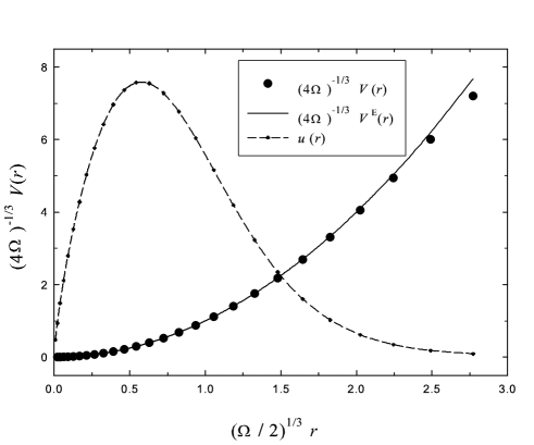
Figure 5: Comparison between the potential computed from the $1S$ wave function (31) with a semirelativistic kinematics (circles) and the exact harmonic potential (solid line) given by Eq. (34). The regularized wave function is also plotted with an arbitrary normalization (dashed line). We used $N=30$, and $(\Omega/2)^{1/3}h=0.034$ from Eq. (33).

is given in Fig. 5. The value $\Omega=0.2$ GeV³ is typical for potential models of light quarks drg . But, we present our results as dimensionless quantities. The curves are thus universal: they do not dependent on $\Omega$, which is the only parameter of this Hamiltonian. Although still satisfactory, the agreement is not as good as with the nonrelativistic applications. We find indeed $\delta=3.1~{}\%$. By inspection of Fig. 5, it can be seen that the last points slightly differ from the exact curve. These points are related to the value of the wave function in its asymptotic tail, as it can be seen from Eq. (11). It means that finding the equivalent potential, especially with a semirelativistic kinematics, needs a good knowledge of the tail, which is not often necessary for computation of the energy spectra.

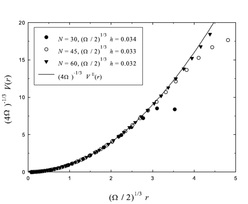
Figure 6: Complete curves giving the potential computed from the $1S$ wave function (31) with a semirelativistic kinematics for several choices of $h$ and $N$. These choices ensure more or less the same mesh point density. The potential is only known at the mesh points (symbols), and the exact harmonic potential is plotted with a solid line.

In our case, the discrepancies for the last points are due to the computation of the wave function in the asymptotic regime. It can be checked that a resolution of Hamiltonian (30) with the Lagrange mesh method leads to a wave function which asymptotically decreases faster than the exact wave function, given by Eq. (31). Conversely, if one starts from the exact wave function, the Lagrange mesh procedure will lead to a potential which does not increase enough asymptotically, as we observe in Fig. 5. Fortunately, only the very last points are affected, as it is shown in Fig. 6. By varying $N$ and $h$, that is to say by varying the interval where the potential is computed, one can always correctly reproduce the potential in a given region: the more $hx_{N}$ is large, the larger is the interval where the potential is correctly reproduced. Finding the equivalent potential with a spinless Salpeter equation seems thus to require a more careful study: several curves have to be computed by varying $h$ and $N$ in order to understand whether the long range behavior of the potential is physical or simply due to a numerical artifact.

VI Conclusions and outlook

In this work, we extended the domain of application of the Lagrange mesh method to a particular type of problem: to find the equivalent local potential corresponding to a given bound state with a given kinematics. We assumed a central problem. Starting from a particular radial wave function and the corresponding energy, the method we presented here allows to compute the equivalent local potential at the mesh points. We checked the accuracy of the computations in various cases whose solutions are analytically known. Firstly, we studied the well-known nonrelativistic harmonic oscillator and Coulomb potentials. These potentials are correctly reproduced by the Lagrange mesh method with a precision better than $1~{}\%$, provided the scale parameter is large enough to take into account the asymptotic tail of the wave function. Moreover, the singularity of the Coulomb potential is well matched. The numerical parameters are the number of mesh points, and the scale parameter. It appears that a typical value of $30$ mesh points is enough to provide a good picture of the potential. As it was the case for usual eigenvalue problems, the scale parameter does not need to be accurately determined: a rather large interval exists where the precision is lower than $1~{}\%$.

If the spectrum comes from a nonlocal potential, our method will compute the equivalent local potential. This problem is of interest in nuclear physics nucl . As an illustration, we applied it to the nonlocal Yamaguchi potential describing the deuteron. In this particular case, the spectrum is analytical as well as the corresponding equivalent potential. Again, the accuracy of our method is very good.

Finally, our procedure can also be easily adapted to the case of a semirelativistic kinematics. As a check, we studied the semirelativistic harmonic oscillator. Again, the potential is correctly reproduced, but it appears that the asymptotic behavior of the potential is problematic. This is an artifact of the method in the semirelativistic case: by varying the mesh size, one can indeed see that the value of the potential at the last mesh points is systematically too low, but the harmonic shape of the potential is well reproduced at the other mesh points.

Our purpose is to apply this method to the study of systems containing quarks and gluons. In particular, glueballs, which are bound states of gluons, are very interesting systems because their existence is directly related to the nonabelian nature of QCD. Bound states of two gluons can be described within the framework of potential models by a spinless Salpeter equation with a Cornell potential: a linear confining term plus a Coulomb term coming from short-range interactions brau . Such a phenomenological potential has been shown to arise from QCD in the case of a quark-antiquark bound state loop . Theoretical indications show that it could be valid also for glueballs simo . Moreover, recently, the mass and the wave function of the scalar glueball (with quantum numbers $J^{PC}=0^{++}$) has been computed in lattice QCD lat . Thanks to the Lagrange mesh method, these data could be used to extract the potential between two gluons from lattice QCD, and see whether it is a Cornell one or not. This study will be published elsewhere.

- (1) D. Baye and P.-H. Heenen, J. Phys. A 19, 2041 (1986).
- (2) M. Vincke, L. Malegat, and D. Baye, J. Phys. B 26, 811 (1993).
- (3) D. Baye, J. Phys. B 28, 4399 (1995).
- (4) M. Hesse, J. Roland, and D. Baye, Nucl. Phys. A 709, 184 (2002).
- (5) C. Semay, D. Baye, M. Hesse, and B. Silvestre-Brac, Phys. Rev. E 64, 016703 (2001).
- (6) F. Brau and C. Semay, J. Phys. G: Nucl. Part. Phys. 28, 2771 (2002) [hep-ph/0412177].
- (7) M. Hesse and D. Baye, J. Phys. B 32, 5605 (1999).
- (8) M. Theeten, D. Baye, and P. Descouvemont, Nucl. Phys. A 753, 233 (2005).
- (9) F. Perey and B. Buck, Nucl. Phys. 32, 353 (1962); A. Lovell and K. Amos, Phys. Rev. C 62, 064614 (2000), and references therein.
- (10) F. Buisseret and C. Semay, Phys. Rev. E 71, 026705 (2005) [hep-ph/0409033].
- (11) D. Baye, M. Hesse, and M. Vincke, Phys. Rev. E 65, 026701 (2002).
- (12) S. Flügge, Practical Quantum Mechanics, Springer, 1999.
- (13) A. De Rùjula, H. Georgi, and S. L. Glashow, Phys. Rev. D 12, 147 (1975); W. Celmaster, Phys. Rev. D 15, 1391 (1977).
- (14) L. Landau and E. Lifchitz, Quantum mechanics, Addison-Wesley, 1958.
- (15) Y. Yamaguchi, Phys. Rev. 95, 1628 (1954).
- (16) W. van Dijk, Phys. Rev. C 40, 1437 (1989).
- (17) R. K. Bhaduri, W. Leidemann, G. Orlandini, and E. L. Tomusiak, Phys. Rev. C 42, 1867 (1990).
- (18) D. LaCourse and M. G. Olsson, Phys. Rev. D 39, 2751 (1989).
- (19) Z.-F. Li, J.-J. Liu, W. Lucha, W.-G. Ma, and F. F. Schöberl, J. Math. Phys. 46, 103514 (2005) [hep-ph/0501268].
- (20) M. Abramowitz and I. A. Stegun, Handbook of mathematical functions, Dover, 1970.
- (21) C. Semay, B. Silvestre-Brac, and I. M. Narodetskii, Phys. Rev. D 69, 014003 (2004) [hep-ph/0309256].
- (22) F. Brau and C. Semay, Phys. Rev. D 70, 014017 (2004) [hep-ph/0412173], and references therein.
- (23) K. G. Wilson, Phys. Rev. D 10, 2445 (1974); N. Brambilla, P. Consoli, and G. M. Prosperi, Phys. Rev. D 50, 5878 (1994).
- (24) A. B. Kaidalov and Yu. A. Simonov, Phys. Lett. B 477, 163 (2000) [hep-ph/9912434].
- (25) P. de Forcrand and K.-F. Liu, Phys. Rev. Lett. 69, 245 (1992); M. Loan and Y. Ying, Prog. Theor. Phys. 116, 169 (2006) [hep-lat/0603030].