Theory of second harmonic generation in colloidal crystals

Abstract

On the basis of the Edward-Kornfeld formulation, we study the effective susceptibility of second-harmonic generation (SHG) in colloidal crystals, which are made of graded metallodielectric nanoparticles with an intrinsic SHG susceptibility suspended in a host liquid. We find a large enhancement and redshift of SHG responses, which arises from the periodic structure, local field effects and gradation in the metallic cores. The optimization of the Ewald-Kornfeld formulation is also investigated.

I Introduction

Nonlinear composite materials with high nonlinear optical susceptibilities or optimal figure of merit (FOM) have drawn considerable attention for their potential applications, e.g., in bistable switches, optical correlators, and so on^1-6. With several advancements in nanotechnology, such as templated sedimentation and dielectrophoresis^7-10, it is possible to fabricate particles with specific geometry. It has also been reported^4,6,11,12 that graded composite materials whose physical properties vary gradually in space^13-16 can exhibit enhanced nonlinear optical responses⁶ and optimal dielectric ac responses¹⁷, as well as conductive responses¹⁸.

It is known that materials lacking inversion symmetry can exhibit a so-called second order nonlinearity¹. This can give rise to the phenomenon of second harmonic generation (SHG), i.e., an input (pump) wave can generate another wave with twice the optical frequency (namely, half the wavelength) in the medium. In most cases, the pump wave is delivered in the form of a laser beam, and the second-harmonic wave is generated in the form of a beam propagating in a similar direction. The physical mechanism behind SHG can be understood as follows. Due to the second order nonlinearity, the fundamental (pump) wave generates a nonlinear polarization which oscillates with twice the fundamental frequency. According to Maxwell’s equations, this nonlinear polarization radiates an electromagnetic field with this doubled frequency. Due to phase matching issues, the generated second-harmonic field propagates dominantly in the direction of the nonlinear polarization wave. The latter also interacts with the fundamental wave, so that the pump wave can be attenuated (pump depletion) when the second-harmonic intensity develops. In the mean time, the energy is transferred from the pump wave to the second-harmonic wave. The SHG effect, like the third-order Kerr-type coefficient, involves the nonlinear susceptibilities of the constituents and local field enhancement which arises from the structure of composite materials^19-23. For example, Hui and Stroud studied a dilute suspension of coated particles with the shell having a nonlinear susceptibility for SHG¹⁹, and Fan and Huang designed a class of ferrofluid-based soft nonlinear optical materials with enhanced SHG with magnetic-field controllabilities²⁰. Both SHG and phase transformation behaviors can be detected in many nanocrystals by using classical methods like X-ray diffraction or Raman spectroscopy^24,25. Until now, achieving enhanced SHG is a challenge^26,27.

Theoretical²⁸ and experimental^29,30 reports also suggested that spherical particles exhibit a rather unexpected and nontrivial SHG due to the broken inversion symmetry at particle surfaces (namely, atoms in the surface occupy positions that lack inversion symmetry), despite their central symmetry which seemingly prohibits second-order nonlinear effects. In colloidal suspensions, the SHG response for centrosymmetric particles was experimentally reported^29,30. Most recently, SHG was also shown to appear for spherical semiconductor nanocrystals³¹. So far, the SHG arising from centrosymmetrical structure has received an extensive attention^28-30,32,33.

Colloidal crystals have been widely studied in nanomaterials and have potential applications in nanophotonics, chemistry, and biomedicine³⁴. For colloidal crystals, the individual colloidal nanoparticles should be touching since the lattice parameters of the crystals, $a$, $b$ and $c$, should satisfy the geometric constraint $a^{2}+b^{2}+c^{2}=16R_{0}^{2}$, where $R_{0}$ denotes the radius of an individual colloidal nanoparticle. However, it is possible to achieve a colloidal crystal without the particles’ touching if the colloidal nanoparticles are charged and stabilized by electrostatic forces. In this work, we shall investigate colloidal crystals with the particles’ touching. Owing to recent advancements in the fabrication of nanoshells^35,36, we are allowed to use a dielectric surface layer with thickness $d$ on a graded metallic core with radius $a_{0}$, in order to activate repulsive or attractive forces between the nanoparticles. The dielectric constant of the metallic core should be a radial function because of a radial gradation, and that of the surface layer can be the same as that of the host liquid, as to be used in this work. The latter is also a crucial requirement because otherwise multipolar interaction between the metallic cores can become important³⁷. In this regard, the surface layer contributes to the geometric constraint, rather than the effective optical responses of the colloidal crystals. In this work, based on the Ewald-Kornfeld formulation [Eq. (7)]³⁸ and the nonlinear differential effective dipole approximation (NDEDA) method [Eq. (LABEL:NDEDA1)]^39,40, we shall focus on the possibility of achieving such colloidal crystals with desired SHG signals.

This paper is organized as follows. In section II, we apply the Ewald-Kornfeld formulation to derive the local electric field in three typical structures of colloid crystals, and then perform the NDEDA method to extract the effective linear dielectric constant and nonlinear susceptibility for SHG. In Section III, we discuss the optimization of the Ewald-Kornfeld summation. Then, we numerically investigate the SHG under different conditions in Section IV, which is followed by a discussion and conclusion in Section V.

II Formalism

Let us start by considering a graded metallic core with radius $a_{0}$ (Fig. 1). When we take into account quadratic nonlinearities only, the local constitutive relation between the displacement field ${\bf D}(r)$ and electric field ${\bf E}(r)$ is given by^41-43

$$D_{i}(r)=\sum_{j}\epsilon_{ij}E_{j}(r)+\sum_{jk}\chi_{ijk}(r)E_{j}(r)E_{k}(r),\,\,i=x,y,z,$$ (1)

where $D_{i}(r)$ and $E_{i}(r)$ are the $i$th component of ${\bf D}(r)$ and ${\bf E}(r)$, respectively, and $\chi_{ijk}$ is the nonlinear susceptibility for SHG. Here $\epsilon_{ij}=\epsilon(r)\delta_{ij}$ denotes the linear dielectric constant, which is assumed for simplicity to be isotropic. Both $\epsilon(r)$ and $\chi_{ijk}(r)$ are functions of $r$, as a result of the gradation profile along the radius $r$ (Fig. 1). If a monochromatic external field is applied, the nonlinearity in the system will generally generate local potentials and fields at all harmonic frequencies. For a finite frequency external electric field along $z-$axis of the form

$$E_{0}=E_{0}(\omega)e^{-i\omega t}+c.c.,$$ (2)

the effective SHG susceptibility $\chi_{2\omega}$ can be extracted by considering the volume average of the displacement field at the frequency $2\omega$ in the inhomogeneous medium^19,41-43. In Eq. (2), $c.c.$ is referred to complex conjugate. The graded metallic core can be built up by adding shells gradually, making the dielectric constant $\epsilon(r)(r\leq a)$ a radial function, which is schematically shown in Fig. 1. We assume that the dielectric constant of the surface and the linear host liquid is a constant for convenience, as mentioned in Section I. At radius $r$, the inhomogeneous spherical particle with $\epsilon(r)$ and $\chi_{2\omega}(r)$ can have the same dipole moment effect as the homogenous sphere with $\bar{\epsilon}(r)$ and $\bar{\chi}_{2\omega}(r)$. The equivalent dielectric constant $\bar{\epsilon}(r)$ can be expressed as the following differential equation obtained from the differential effective dipole approximation method^13,39,

$$\frac{d\bar{\epsilon}(r)}{dr}=\frac{(\epsilon(r)-\bar{\epsilon}(r))(\bar{\epsilon}(r)+2\epsilon(r))}{r\epsilon(r)}.$$ (3)

On the other hand, the equivalent susceptibility for SHG $\bar{\chi}_{2\omega}(r)$ can be written as⁴⁰

$$\frac{d\bar{\chi}_{2\omega}(r)}{dr} = \bar{\chi}_{2\omega}(r)\left(\frac{2d\bar{\epsilon}_{\omega}(r)/dr}{2\epsilon_{2}+\bar{\epsilon}_{\omega}(r)}+\frac{d\bar{\epsilon}_{2\omega}(r)/dr}{2\epsilon_{2}+\bar{\epsilon}_{2\omega}(r)}+\frac{2y(\omega,r)+y(2\omega,r)-3}{r}\right)$$

$$+3\chi_{2\omega}(r)\left(\frac{[x^{2}(\omega,r)+\frac{28}{35}z^{2}(\omega,r)]x(2\omega,r)+\frac{8}{35}[7x(\omega,r)+2z(\omega,r)]z(\omega,r)z(2\omega,r)}{rf(2\omega,r)f^{2}(\omega,r)}\right),$$

where $x(\omega,r)=\frac{\epsilon_{2}(r)(\bar{\epsilon}_{\omega}(r)+2\epsilon_{\omega}(r))}{\epsilon_{\omega}(r)(\bar{\epsilon}_{\omega}(r)+2\epsilon_{2}(r))},$ $y(\omega,r)=2\frac{(\bar{\epsilon}_{\omega}(r)-\epsilon_{\omega}(r))(\epsilon_{\omega}(r)-\epsilon_{2}(r))}{\epsilon_{\omega}(r)(\bar{\epsilon}_{\omega}(r)+2\epsilon_{2}(r))},$ $z(\omega,r)=\frac{\epsilon_{2}(r)(\bar{\epsilon}_{\omega}(r)-\epsilon_{\omega}(r))}{\epsilon_{\omega}(r)(\bar{\epsilon}_{\omega}(r)+2\epsilon_{2}(r))},$ and $f(\omega,r)=\frac{3\epsilon_{2}(r)}{\bar{\epsilon}_{\omega}(r)+2\epsilon_{2}(r)}$. Here the indices $\omega$ and $2\omega$ correspond to basic and second harmonics for the nonlinear susceptibility, respectively, and $\bar{\chi}_{2\omega}(r)$ denotes the equivalent SHG susceptibility of the whole graded spherical particle with radius $r$. For convenience, we shall denote $\bar{\chi}_{2\omega}(r=a)$ as $\bar{\chi}_{2\omega}$ in the following.

The above two differential equations [Eqs. (3)-(LABEL:NDEDA1)] can be solved numerically as long as the gradation profiles are given. For obtaining the effective dielectric constant of the colloidal crystal, we refer to the Maxwell-Garnett approximation⁴⁴

$$\frac{\epsilon_{e}-\epsilon_{2}}{\alpha\epsilon_{e}+(3-\alpha)\epsilon_{2}}=\rho\frac{\bar{\epsilon}-\epsilon_{2}}{\bar{\epsilon}+2\epsilon_{2}},$$ (5)

where $\rho$ denotes the volume fraction of the metallic component [see Eq. (6)], and the local field factor $\alpha$ represents $\alpha_{\perp}$ (transverse field cases) and $\alpha_{\parallel}$ (longitudinal field cases), respectively. Here the longitudinal (or transverse) field case corresponds to the fact that the $E$ field of the incident light is parallel (or perpendicular) to the uniaxial anisotropic axis. For $\alpha_{\perp}$ and $\alpha_{\parallel}$, there is a sum rule $2\alpha_{\perp}+\alpha_{\parallel}=3$ ^45,46. Next, we shall apply the Ewald-Kornfeld model to compute the local field factor $\alpha$ for a tetragonal unit cell that can be viewed as a tetragonal lattice plus a basis of two nanoparticles. One of the two nanoparticles is located at the corner of the cell, and the other is at the body center. Without loss of generality, we consider three representative lattices (Fig. 2): the bct (body-centered tetragonal), bcc (body-centered cubic) and fcc (face-centered cubic) lattice. If the uniaxial anisotropic axis is directed along the $z$ axis, the lattice constants can be denoted by $a(=b)=\ell q^{-\frac{1}{2}}$ along ${\bf x}$ (${\bf y}$) axis and $c=\ell q$ along ${\bf z}$ axis, and the volume of the unit cell $V_{c}=\ell^{3}.$ The lattice parameters satisfy the geometric constraint that $a^{2}+b^{2}+c^{2}=16(a_{0}+d)^{2}$, when we take into account the dielectric surface layer with thickness $d$ on the graded metallic core. It is easy to obtain the value of $q$ from their intrinsic structures: $\textit{q}=0.87358,1.0$ and $2^{\frac{1}{3}}$ represent the bct, bcc and fcc lattice, respectively. Table 1 shows the calculated values of $\alpha_{\perp}$ and $\alpha_{\parallel}$ versus $q$, according to Eq. (7) below. The degree of anisotropy of the periodic lattices is measured by how $q$ deviates from unity. Here we assume that the colloidal particles are packed closely together. Meanwhile, we obtain a relation between $q$ and the volume fraction $\rho$ of the metallic component,

$$\rho=\frac{\pi}{24t^{3}}\sqrt{\left(\frac{q^{3}+2}{q}\right)^{3}},$$ (6)

with thickness parameter $t=(a_{0}+d)/a_{0}$, $t>1$. The lattice vector of the tetragonal lattice is given by ${\bf R}=\ell(q^{-\frac{1}{2}}l\hat{{\bf x}}+q^{-\frac{1}{2}}m\hat{{\bf y}}+qn\hat{{\bf z}}),$ where $l,$ $m,$ and $n$ are integers. When an external electric field $\mathbf{E_{0}}$ is applied along the ${\bf x}$ axis, the induced dipole moment ${\bf p}$ are perpendicular to the uniaxial anisotropic axis. Considering the field contribution from all the other particles in the lattice, the local field $\mathbf{E_{L}}$ at the lattice point ${\bf r}={\bf 0}$ can be given as

$$E_{L}=p\sum_{j=1}^{2}\sum_{{\bf R}\neq{\bf 0}}[-B(R_{j})+x_{j}^{2}q^{2}C(R_{j})]-\frac{4\pi p}{V_{c}}\sum_{{\bf G}\neq{\bf 0}}\Theta({\bf G})\frac{G_{x}^{2}}{G^{2}}\exp\left(\frac{-G^{2}}{4\eta^{2}}\right)+\frac{4p\eta^{3}}{3\sqrt{\pi}},$$ (7)

where $x_{j}=l-(j-1)/2$, $R_{j}=|{\bf R}-[(j-1)/2](a\hat{{\bf x}}+b\hat{{\bf y}}+c\hat{{\bf z}})|,$ and $\Theta({\bf G})=1+\exp[i(u+v+w)/\pi].$ In Eq. (7), $B$ and $C$ are two coefficients given in⁴⁶, $B(r)=\textmd{erfc}(\eta r)/r^{3}+2\eta/(\sqrt{\pi}r^{2})\exp(-\eta^{2}r^{2}))$ and $C(r)=3\textmd{erfc}(\eta r)/r^{5}+[4\eta^{3}/(\sqrt{\pi}r^{2})+6\eta/(\sqrt{\pi}r^{4})]\exp(-\eta^{2}r^{2})$, where $\textmd{erfc}(\eta r)$ is the complementary error function and $\eta$ is an adjustable parameter making the summation converge rapidly. For details, please see Section III. In Eq. (7), $p$ denotes the strength of the induced dipole moment, and ${\bf G}$ the reciprocal lattice vector of ${\bf R}$. Thus the local field factor in transverse fields can be defined as

$$\alpha_{\perp}=\frac{3}{4\pi}\frac{V_{c}E_{L}}{p}.$$ (8)

For the bct, bcc and fcc lattices, we obtain $\alpha_{\bot}=0.95351,1.0$ and $1.0,$ respectively. Following refs 19 and 20, the effective SHG susceptibility of the whole system $\chi_{2\omega}$ is given by

$$\chi_{2\omega}=\rho\bar{\chi}_{2\omega}\Gamma(2\omega)\Gamma^{2}(\omega),$$ (9)

where $\Gamma(\omega)$ denotes the factor in a linear system which, for consistency with Eq. (5) in getting $\epsilon_{e}$, should also be determined by using the Maxwell-Garnett approach. Thus, we obtain

$$\Gamma(\omega)=\frac{3\epsilon_{2}}{(1-\rho\alpha)\bar{\epsilon}(\omega)+(2+\rho\alpha)\epsilon_{2}}.$$ (10)

Meanwhile, $\bar{\chi}_{2\omega}$ can be obtained through the NDEDA method [Eq. (LABEL:NDEDA1)].

III Optimization of the Ewald-Kornfeld summation [Eq. (7)]

In Eq. (7), we see the adjustable parameter $\eta$ dominates the accuracy and the efficiency of the Ewald-Kornfeld summation^46,47. An important aspect of the Ewald-Kornfeld summation is the tuning in the sense of speed at well controlled errors. It should be chosen carefully in order to make the summations both in the real space and the reciprocal lattices converge rapidly^46-48. On the other hand, the $r$-space cutoff $r_{c}$ and the $k$-space cutoff $k_{c}$ are also difficult to be determined^46-48. In this section, we shall analyze the role of these 3 parameters, especially on lattices depicted in Fig. 2. Similarly, it can also be applied to other lattice models.

In condensed matter physics, complex dielectrics should obey the famous sum rule $\beta_{x}+\beta_{y}+\beta_{z}=4\pi$, where $\beta_{x},$ $\beta_{y},$ and $\beta_{z}$ are the local field factors along $x,$ $y,$ and $z$ axes, respectively [Eq. (11)]. We shall use this rule to estimate the accuracy of our algorithm.

First of all, let us investigate how the lattice parameters affect the accuracy of calculation. We test 4 lattices with $\{a=1,b=1,c=1,5,10\}$ and $\{a=10,b=10,c=10\}$ respectively. The cutoffs in the $r-$ and $k-$ spaces are fixed to 3 which means that we take summation over 6 periods in each direction. By using the relation mentioned above, we have

$$\beta_{i}=\frac{E_{L,i}({\bf p}_{i})V_{c}}{2p_{i}}\equiv\frac{4\pi}{3}\alpha,$$ (11)

where the subscript $i$ stands for Cartesian directions $x,$ $y,$ and $z.$ The local-field factors $\alpha$ [Eq. (5)] and $\beta$ [Eq. (11)] have exactly the same concept, the only difference is that there is a proportionality constant $4\pi/3$ between $\beta$ and $\alpha$, as shown in [Eq. (11)]. In detail, $\alpha_{\perp}=(4\pi/3)\beta_{x}$ or $(4\pi/3)\beta_{y}$, and $\alpha_{\|}=(4\pi/3)\beta_{z}$.

Next, let us plot the result of the Ewald-Kornfeld summation vs splitting parameter in Fig. 3. The total local field factor $\beta_{total}=\beta_{x}+\beta_{y}+\beta_{z}$ is normalized by $4\pi.$ When $\{{a=b=c=1}\}$, there is a wide platform with $\eta$ goes from 1 to 3. In this case, the correctness of our algorithm can be guaranteed by choosing $\eta$ with any value within the platform region. However, as ${c}$ increases, the anisotropic degree becomes strong, and the original platform rapidly shortens. In the lattice $\{{a=b=1,c=5}\}$, the proper region of $\eta$ only has the width 0.25. Further, in the lattice $\{{a=b=1,c=10}\}$, the platform even disappears. At that time, the correct result could not be achieved if we would not adjust $r_{c}$ and $k_{c}$. Another isotropic lattice $\{{a=b=c=10}\}$ is also investigated. Although the shape of the figure is similar with that of $\{{a=b=c=1}\}$, the platform is remarkably shrunk.

Then, let us see how the shape of summation region affects the accuracy. For highly anisotropic lattices, i.e. $\{{a=b=1,c=10}\}$, the method of cubic region summation is not applicable because it counts in many source sites far from the field point along the uniaxial direction, but ignores many sites near the field point in the other two isotropic direction (see Fig. 4). It may be improved by using a spherical region summation. Set $l,$ $m,$ and $n$ to be sum indices in $r-$space, and $u,$ $v,$ and $w$ to be in $k$-space. For the cubic region summation, we just require all these indices to be within [-maximum, maximum]. But for the spherical region summation, the requirement turns out to be

$$(al)^{2}+(bm)^{2}+(cn)^{2}\leq R_{r}^{2},$$ (12)

$$(u/a)^{2}+(v/b)^{2}+(w/c)^{2}\leq R_{k}^{2}.$$ (13)

Figure 5 shows the effect of such spherical region summation. The circle line is obtained by imposing the restriction that all summation indices are within [-5,5], and the star line is obtained by using the spherical region summation. The maximum radii, $R_{r}$ [Eq. (12)] and $R_{k}$ [Eq. (13)], are the length of the diagonal of the unit cell in $r-$ and $k-$space, respectively,

$$(al)^{2}+(bm)^{2}+(cn)^{2}\leq a^{2}+b^{2}+c^{2}=R_{r}^{2},$$ (14)

$$(u/a)^{2}+(v/b)^{2}+(w/c)^{2}\leq(1/a)^{2}+(1/b)^{2}+(1/c)^{2}=R_{k}^{2}.$$ (15)

This summation region is smaller than the cubic region, and less sites are evaluated naturally. Nevertheless, a wider platform is achieved for this region. The main reason is that the spherical region summation tends to count in the sites which contribute much to the field point. The two lines in Fig. 5 show the same value when $\eta$ becomes larger. Later we shall see that this is due to the result in the $k$-space summation that is not modified too much.

Last, we demonstrate how $r_{c}$ and $k_{c}$ affect the accuracy. In general, the larger radii the cutoff has, the more precise the result is. Unfortunately, larger summation regions cost longer computation time. Thus, we should take optimized values of $r_{c}$ and $k_{c}$. In Fig. 6, we calculate the total local field factor for four configurations of cutoffs. The left-top graph is copied from Fig. 5. Meanwhile, the right-bottom plot is obtained with twice value of $r_{c}$ and $k_{c}$. We find that by increasing $r_{c}$, the platform would extend to the left with the limit of zero, but there is no such limit by increasing $k_{c}$. As $k_{c}$ increases, the platform could extend to the wide space on the right.

In conclusion, in order to optimize the Ewald-Kornfeld summation [Eq. (7)], we had better perform the sum in a spherical shape. Enlarging the summation radius in $k$-space is more efficient than that in $r$-space. Our method might test the sum rule first with a large enough $r_{c}$ and $k_{c}$ (here time is not the main concern), and then it is convenient for one to choose the center value of $\eta$ in the platform. This guarantees the correctness of all the computations performed for achieving Table 1.

IV Numerical Results

For numerical calculations, we set the linear dielectric constant of the nonlinear metallic core to have the following Drude form

$$\epsilon(r)=1-\frac{\omega_{p}(r)^{2}}{\omega(\omega+i\gamma)},$$ (16)

where $\omega_{p}(r)$ means a position-dependent plasma frequency, and $\gamma$ relaxation rate. For achieving the position-dependent plasma frequency, one possible way is to fabricate metallic spherical particles containing multilayers each of which is made of different metals. For numerical calculations, we take a model plasma-frequency gradation profile

$$\omega_{p}(r)=\omega_{p}(0)\left(1-C_{\omega}\frac{r}{a}\right),$$ (17)

where $C_{\omega}$ is a parameter adjusting the gradation profile. For focusing on the enhancement of the SHG response, we take the intrinsic nonlinear SHG susceptibility $\chi_{1}$ to be a frequency-and-position independent real positive constant.

Figure 7 shows (a) the imaginary part of the effective linear dielectric constant (namely, optical absorption), (b) the real and (c) imaginary parts of the effective SHG susceptibility, (d) the modulus of $\bar{\chi}_{2\omega}/\chi_{1}$, and (e) the FOM (figure of merit) as a function of frequency for longitudinal field cases. As $C_{\omega}$ increases, $\omega_{p}(r)$ takes on a broader range of value and leads to a broad plasmon band, while the plasmon peak shifts to lower frequencies (namely, redshift). The susceptibility of the SHG also shows an enhancement and the peak of enhancement can be shifted to lower frequencies, too. Generally, the SHG susceptibility and FOM can be enhanced in some frequency regions as $C_{\omega}$ increases.

Figure 8 shows the effective responses and FOM as a function of thickness parameter $t$, for bct lattices. For the given lattice it is evident that the effective linear and nonlinear optical responses strongly depend on the thickness parameter. Both the redshift and strength of the plasma resonant peak are largest at the smallest $t$ for linear optical absorption. In this case, the plasma resonant band is also largest for smallest $t$. Similar behavior can also be found for the nonlinear SHG responses. On the other hand, $t$ has an effect on the FOM, too. All of these results come from the combination of gradation, local fields, and periodic lattice effects. In fact, the volume fraction for different colloidal lattices also contributes to the nature of plasma resonant. For the fcc lattice, its redshift may lie between bct and bcc lattices, and for the current parameters in use, its deference between fcc and bcc (or bct) is smaller than 4% (no pictures shown here). It can also be found that as $t$ increases (or, alternatively the colloid crystals become more dilute), the behavior of plasma resonant becomes more similar. This can be explained from the dilute limit approximation model for the enhancement of optical susceptibility.

In Figs. 7 and 8 the quantities that can be both positive and negative are plotted in a logarithm of modulus. When the quantities pass through zero, the logarithm is very large, thus yielding spikes. In addition, we can reach the conclusion that the FOM in the high frequency region is still attractive due to the presence of weak optical absorption.

V Discussion and conclusion

Our main idea is to first reduce the graded metallic cores to effective ones and then consider colloidal crystals consisting of such effective nanoparticles embedded in a host liquid that has the same dielectric constant as the dielectric shells of the nanoparticles. In doing so , multipolar interaction between the metallic cores can become unimportant for arbitrary field polarizations. It should be remarked that, since the nonlinear response will depend on the local fields and nonlinear susceptibility tensors in the whole structure (due to the broken symmetry at the surface of the metallic core), the response can be tensorial and variant within the core. In this work we have treated the quantities as a scalar and constant, in order to focus on the effects of lattices and gradation of our interest.

As the value of $q$ increases, the responses in transverse field will have slight difference from the longitudinal case (no figures shown here), because of the little difference between $\alpha_{\bot}$ and $\alpha_{\|}$ for a given structure. From bct, bcc to fcc lattices, with the increase of $q$ , the longitudinal local field factor $\alpha_{\|}$ decreases from 1.09299 at bct lattices to 1.0 at bcc and fcc lattices, while the volume fraction $p$ decreases to bcc, then increases to fcc. This trend can also be seen in other bulk samples, such as rhombohedral, orthorhombic and hexagonal.

We have investigated the cases of graded plasma frequencies, by assuming the relaxation rate $\gamma$ to be a constant. In fact, $\gamma$ can also be inhomogeneous. For instance, a position-dependent profile for the relaxation rate can be achieved experimentally. One possible way may be to fabricate dirty metallic spherical particles in which the degree of disorder varies in the radial direction and hence leads to a relaxation-rate gradation profile. In case of graded relaxation rates, the nonlinear optical responses can also be adjusted by choosing appropriate gradation profiles for relaxation rates¹¹.

Throughout the paper, the host medium is assumed to be isotropic. It is interesting to see what will happen if the host is anisotropic, e.g., for a graded-index host⁴⁹. In this case, the gradation is also expected to yield desired enhanced SHG. On the other hand, optical switching in graded plasmonic crystals via nonlinear pumping was recently reported⁵⁰, which might also be realized in graded colloidal crystals proposed in this work.

In summary, based on the Edward-Kornfeld formulation, we have theoretically exploited a class of nonlinear materials possessing a nonvalishing SHG susceptibility, which are based on colloidal crystals of graded metallodielectric nanoparticles. They have been shown to have an enhancement and redshift of SHG signals due to the combination of various effects.

References and notes

(1) Shen, Y. R. The Principles of Nonlinear Optics; Wiley: New York, 1984.

(2) Boyd, R. W. Nonlinear Optics; Academic: New York, 1992.

(3) Rodenberger, D. C.; Heflin, J. R.; Garito, A. F. Nature (London) 1992, 359, 309.

(4) Fischer, G. L.; Boyd, R. W.; Gehr, R. J.; Jenekhe, S .A.; Osaheni, J. A.; Sipe, J. E.; Weller-Brophy, L. A. Phys. Rev. Lett. 1995, 74, 1871.

(5) Sekikawa, T.; Kosuge, A.; Kanai, T.; Watanabe, S. Nature (London) 2004, 432, 605.

(6) Huang, J. P.; Yu, K. W. Phys. Rep. 2006, 431, 87.

(7) Blaaderen, A. V. MRS Bull. 2004, 29, 85.

(8) Velikov, K. P.; Christova, C. G.; Dullens, R. P. A.; van Blaaderen, A. Science 2002, 296, 106.

(9) Gong T.; Marr, D. W. Appl. Phys. Lett. 2004, 85, 3760.

(10) Schilling T.; Frenkel, D. Phys. Rev. Lett. 2004, 92, 085505.

(11) Huang J. P.; Yu, K. W. Appl. Phys. Lett. 2004, 85, 94.

(12) Bennink, R. S.; Yoon, Y.-K.; Boyd, R. W.; Sipe, J. E. Opt. Lett. 1999, 24, 1416.

(13) Milton, G. W. The Theory of Composites; Cambridge University Press: Cambridge, 2002; Chap. VII.

(14) Fan, C. Z.; Huang, J. P.; Yu, K. W. J. Phys. Chem. B 2006, 110, 25665.

(15) Wei, E. B.; Song, J. B.; Gu, G. Q. J. Appl. Phys. 2004, 95, 1377.

(16) Sang Z. F.; Li, Z. Y. Opt. Commun. 2006, 259, 174.

(17) Wei, E. B.; Dong, L.; Yu, K. W. J. Appl. Phys. 2006, 99, 054101.

(18) Gu, G. Q.; Yu, K. W. J. Appl. Phys. 2003, 94, 3376.

(19) Hui P. M.; Stroud, D. J. Appl. Phys. 1997 82, 4740.

(20) Fan C. Z.; Huang, J. P. Appl. Phys. Lett. 2006, 89, 141906.

(21) Reis, H. J. Chem. Phys. 2006, 125, 014506.

(22) Nappa, J.; Russier-Antoine, I.; Benichou, E.; Jonin, C.; Brevet, P. F. J. Chem. Phys. 2006, 125, 184712.

(23) Shalaev, V. M. Phys. Rep. 1996, 272, 61.

(24) Chiang, H. P.; Leung, P. T.; Tse, W. S. J. Phys. Chem. B 2000, 104, 2348.

(25) Han, J.; Chen, D.; Ding, S.; Zhou, H.; Han, Y.; Xiong, G.; Wang, Q. J. Appl. Phys. 2006 99, 023526.

(26) Pezzetta, D.; Sibilia, C.; Bertolotti, M.; Ramponi, R.; Osellame, R.; Marangoni, M.; Haus, J. W.; Scalora, M.; Bloemer, M. J.; Bowden, C. M. J. Opt. Soc. Am. B 2002, 19, 2102.

(27) Purvinis, G.; Priambodo, P. S.; Pomerantz, M.; Zhou, M.; Maldonado, T. A.; Magnusson, R. Opt. Lett. 29, 1108.

(28) Dadap, J. I.; Shan, J.; Eisenthal, K. B.; Heinz, T. F. Phys. Rev. Lett. 1999 83, 4045.

(29) Yang, N.; Angerer, W. E.; Yodh, A. G. Phys. Rev. Lett. 2001, 87, 103902.

(30) Jen, S. H.; Dai, H. L. J. Phys. Chem. B 2006, 110, 23000.

(31) Son, D. H.; Wittenberg, J. S.; Banin, U.; Alivisatos, A. P. J. Phys. Chem. B 2006, 110, 19884.

(32) Xu, P.; Ji, S. H.; Zhu, S. N.; Yu, X. Q.; Sun, J.; Wang, H. T.; He, J. L.; Zhu, Y. Y.; Ming, N. B. Phys. Rev. Lett. 2004, 93, 133904.

(33) Bernal R.; Maytorena, J. A. Phys. Rev. B 2004, 70, 125420.

(34) Colloids and Colloid Assemblies; edited by Caruso, F.; Wiley-VCH: Weinheim, 2004.

(35) Nehl, C. L.; Grady, N. K.; Goodrich, G. P.; Tam, F.; Halas, N. J.; Hafner, J. H. Nano Lett. 2004, 4, 2355.

(36) Mitzi, D. B.; Kosbar, L. L.; Murray, C. E.; Copel, M.; Afzali, A. Nature (London) 2004, 428, 299.

(37) Huang, J. P.; Yu, K. W. Appl. Phy. Lett. 2005, 87, 071103.

(38) Ewald, P. P. Ann. Phys. (Leipzig) 1921, 64, 253; Kornfeld, H. Z. Phys. 1924, 22, 27.

(39) Gao, L.; Huang, J. P.; Yu, K. W. Phys. Rev. B 2004, 69, 075105, and references therein.

(40) Gao, L.; Yu, K. W. Phys. Rev. B 2005, 72, 075111. Although this reference presents all components for an effective nonlinear susceptibility of SHG, in our work, for simplicity, we only perform numerical calculations on the $z$ component, thus yielding eq 4.

(41) Hui, P. M.; Xu, C.; Stroud, D. Phys. Rev. B 2004, 69, 014202.

(42) Hui, P. M.; Xu, C.; Stroud, D. Phys. Rev. B 2004, 69, 014203.

(43) Huang, J. P.; Hui, P. M.; Yu, K. W. Phys. Lett. A 2005, 342, 484.

(44) Lo, C. K.; Wan, J. T. K.; Yu, K. W. J. Phys.: Condens. Matter 2001, 13, 1315.

(45) Landau, L. D.; Lifshitz, E. M.; Pitaevskii, L. P. Electrodynamics of Continuous Media; 2nd ed.; Pergamon: New York, 1984; Chap. II.

(46) Lo, C. K.; Yu, K. W. Phys. Rev. E 2001, 64, 031501.

(47) Shen, L. Dynamic electrorheological effects of rotating spheres; MPhil thesis; Chinese University of Hong Kong: Hong Kong, 2005.

(48) Wang, Z.; Holm, C. J. Chem. Phys. 2001, 115, 6351.

(49) Xiao, J. J.; Yu, K. W. Appl. Phys. Lett. 2006, 88, 071911.

(50) Xiao, J. J.; Yakubo, K.; Yu, K. W. Appl. Phys. Lett. 2006, 88, 241111.

Table 1: Values of $\alpha_{\perp}$ and $\alpha_{\parallel}$ computed at different $q$. $q=0.87358,$ $1,$ and $2^{1/3}$ correspond to bct, bcc, and fcc lattices, respectively.

q	$\alpha_{\perp}$	$\alpha_{\parallel}$
0.87358	0.953506	1.09299
0.9	0.971231	1.05754
1.0	1	1
1.1	0.999345	1.00131
1.2	0.996275	1.00745
$2^{1/3}$	1	1
1.3	1.00601	0.987988
1.4	1.03492	0.930155
1.5	1.08376	0.832478
1.6	1.15032	0.699352
1.7	1.23137	0.537268
1.8	1.32368	0.352638
1.9	1.42459	0.150817

Figure captions

Fig. 1. Schematic graph showing the graded metallic core with radius $a_{0}$ embedded in a linear host liquid. The metallic core has a dielectric shell that has the same dielectric constant as the host liquid, and the core can be built up by adding shells gradually. $\epsilon_{2}$ denotes the linear dielectric constant of the host liquid and shell, and $\epsilon(r)$ is the radius-dependent dielectric constant of the graded metallic core.

Fig. 2. Schematic graph showing unit cells of (a) bct, (b) bcc, and (c) fcc lattices with lattice constants $a$, $b$, and $c$, which satisfy $a(=b)=\ell q^{-1/2}$ and $c=\ell q$. Here, $q=0.87358$ (bct), $1.0$ (bcc), and $2^{1/3}$ (fcc).

Fig. 3. Normalized total local field factors versus splitting parameters in different lattices. The $\eta$ corresponding to $\beta_{{\rm total}}/(4\pi)=1$ leads to accurate result of the Ewald-Kornfeld summation [Eq. (7)].

Fig. 4. Cubic and spherical summation region for lattices with different anisotropic degree.

Fig. 5. Normalized total local field factors versus splitting parameters in cubic and spherical region summation. The platform for the $\eta$ corresponding to $\beta_{{\rm total}}/(4\pi)=1$ is widened by using spherical region summation.

Fig. 6. Normalized total local field factors versus splitting parameters for various $r_{c}$ and $k_{c}$ cutoffs. Increasing $r_{c}$ or $k_{c}$ yields the left or right extension of the platform of the $\eta$ that corresponds to $\beta_{{\rm total}}/(4\pi)=1$, respectively.

Fig. 7. For the bct lattice (longitudinal field), (a) the linear optical absorption Im[$\epsilon_{e}(\omega)$], (b) Im[$\chi_{2\omega}/\chi_{1}$], (c) Re[$\chi_{2\omega}/\chi_{1}]$, (d) modulus of $\chi_{2\omega}/\chi_{1}$, and (e) the FOM=$|\chi_{2\omega}|/[\chi_{1}{\rm Im}(\epsilon_{e})]$ versus the normalized incident angular frequency of $\omega/\omega_{p}(0)$ for the dielectric function gradation profile [Eq. (16)] with various plasma-frequency gradation profiles [Eq. (17)]: $C_{\omega}=0.3,$ $0.5,$ and $0.7.$ Here $|\cdots|$ denotes the absolute value or modulus of $\cdots$. Parameters: $\gamma=0.02\omega_{p}(0),$ $t=3,$ and $\epsilon_{2}=2.25$.

Fig. 8. Same as Fig. 7, but for different thickness $t=1.2,$ $2.0,$ and $3.0.$ Parameters: $\gamma=0.02\omega_{p}(0)$, $C_{\omega}=0.5,$ and $\epsilon_{2}=2.25$.

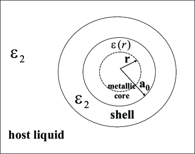
Figure 1: /Huang, Jian, Fan, and Yu

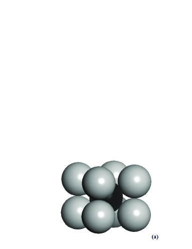
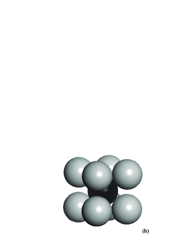
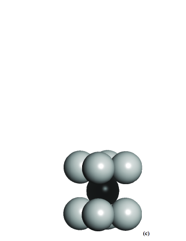
Figure 2: /Huang, Jian, Fan, and Yu

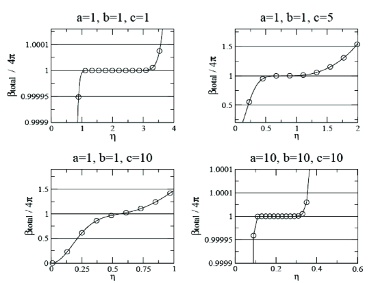
Figure 3: /Huang, Jian, Fan, and Yu

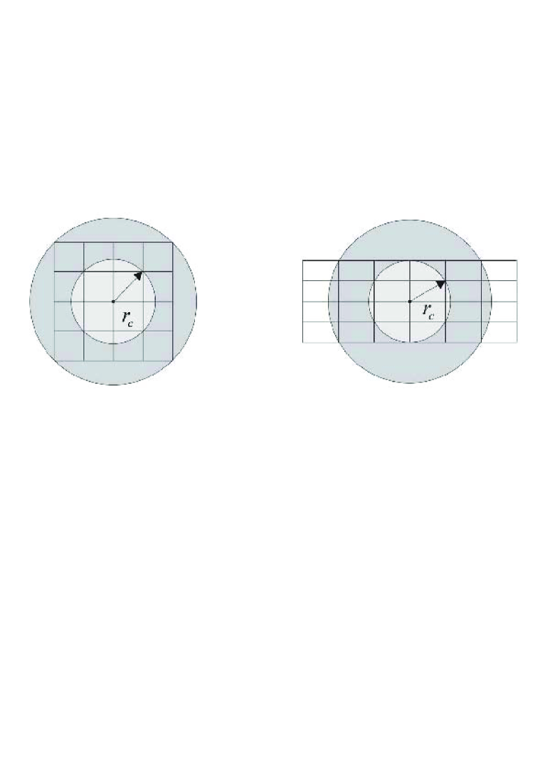
Figure 4: /Huang, Jian, Fan, and Yu

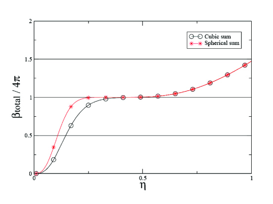
Figure 5: /Huang, Jian, Fan, and Yu

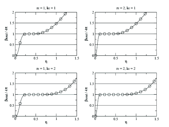
Figure 6: /Huang, Jian, Fan, and Yu

Figure 7: /Huang, Jian, Fan, and Yu

Figure 8: /Huang, Jian, Fan, and Yu