Magnetophoresis of ferrofluid in microchannel system and its nonlinear effect

Abstract

We have studied the magnetophoretic particle separation and its nonlinear behavior of ferrofluids in microchannel which is proposed by Furlani. The magnetic gradient force is caused by an bias field and the polarized magnets and is found to be spatially uniform in the channel section which can be used for particle selecting or separation. We have derived the equations of nonlinear magnetization of magnetic particles which cause the harmonics of magnetophoresis. The Langevin model and generalized Clausius-Mossotti equation used show how the normal and longitude anomalous anisotropic effect the permeability of ferrofluids, thus the magnetic force. Our analysis demonstrates the viability of using the microchannel system for various bioapplications and other characterization of fluid transporting and the time-varying magnetic field can be potentially used for an integrated magnetometer and influences the the viscosity and effective permeability in ferrofluids.

I Introduction

Nowadays magnetophoretic microsystems have been paid great attention in bio-technology for the integration of ”micro-total-analysis”($\mu$TAS) verpoorte because of its high degree of detection and selectivity. The biomaterials possessing low magnetic susceptibility can cause substantial contrast between the labeled and unlabled materials furlani . Because of its polarization difference, the the particles exhibit rich fluid-dynamic behaviors such as magnetophoresis as well as various magnetic responses. Magnetic cell separation can be applied using magnetic beads which coated with specific cell(core-shell microsphere), or the native magnetic susceptibility bizdoaca ; austin . In some special cases such as blood cells, the red and white blood cells can be conducted using magnetophoretic separation based on their native magnetic properties: diamagnetic or paramagnetic han . Magnetic changes in red blood cells can also be used for separation of diseased cells paul . In such continuous microseparator, the ferromanetic wire(circular or square) put in close proximity under an external bias field cause strong magnetic field with high magnetic gradience. Miniaturized Cell separator can be integrated for various types of cell counting and collecting. The magnetophorsis with integrated soft magnetic elements have some advantages over electrophoresis with electromagnets choi for they consume no heat and cause no damage and other negative effect on the bio-cells. Furlani have recently demonstrated transport and capture behavior of magnetic particles such as Fe₃O₄ in the microsystem which consists of an array of integrated soft magnetic elements embedded under the microfluidic channel with also an external bias field. The elements can be polarized by the bias field, thus producing nonuniform field distribution which causes magnetophoretic force on magnetic particles within microchannel. The cubic soft magnetic elements replace the wire, producing different separation and trap in geometry.

In the present paper we emphasize on the characteristics of the magnetic composites(such as large magneticc constants and permanent moments) on the behavior of magnetophoresis in ferrofluids and donot consider the equations for particle motion. In experiment the slow-moving transport is influenced by the viscous drag and thermal kinetics, thus the magnetic force can be measured in the quasi-equilibrium movement.

Ferrofluids(or magnetic fluids) are colloidal suspensions containing single domain nanosized ferromagnetic particles dispersed in a carrier fluid skjeltorp . Since these particles can interact easily and form crystal-like structure in the presence of applied bias magnetic fields, which in turn can affect the viscosity and structural properties tremendously huang , particles in ferrofluids have a wide variety of potential biomedical applications such as label and manipulate biomaterials. The dynamic(ac) magnetic properties and magnetization-induced second-order harmonic generation are taken into consideration in the system. In experiment, the measurement of an ac complex magnetic susceptibility of magnetic fluids is a suitable method to study the relaxation process of the magnetic dipoles of colloidal particles in magnetic fluids zhang ; valenzuela . The second-order harmonic generation is the phenomenon that the magnetization along the specific direction activates the originally silent tensor components for the second-order nonlinear optical susceptibility and is observed for surfaces or interfaces of ferromagnetic materials(thin films) bennemann , or polar antiferromagnets frohlich and polar ferromagnets ogawa .

The saturation of magnetic particles considered here will be different from Furlani’s theory and Han $et$ $al$’s experiment, which cause the nonlinearity to appear by two effects: normal saturation and anomalous saturation. In detail, the normal saturation arises from the higher orders of Langevin function at large filed region, and the anomalous saturation results from the particle chains with higher and lower dipole moments bottcher which is shifted under the influence of the field. The magnetic field inside the ferrofluid plays important role in the coupling between the two effects, which is similar in electrorheological and magnetorheological fluids. When suspension having nonlinear characteristic is subjected to ac magnetic field, the harmonics of magnetic susceptibility can be induced to appear levy . Our analysis demonstrates that the magnetic force will cause suitable separation across microchannel and will be affected by the anisotropic changes of magnetic dipole arrays.

II Theory and Formalism

II.1 Nonlinear magnetic moments in ferrofluids

In the standard case the magnetic induction B is proportional with the field strength $\textbf{H}_{0}$, and have the relation $\textbf{B}=\mu\textbf{H}_{0}$, where $\mu$ is the linear permeability. At strong field intensities, nonlinearities are introduced as ${\bf B}=\mu_{e}{\bf H}_{0}+\chi H_{0}^{2}{\bf H}_{0}$ where third-order and higher-order nonlinear coefficients are dropped and $\chi$ and $\mu_{e}$ are the nonlinear magnetic susceptibility and effective permeability for the longitudinal field case. Here we assume the nonlinearity is not strong and consider only the lowest-order nonlinearity for simplicity.

In the ferrofluids, the average component in the direction of the field of the magnetic dipole moments can be expressed as $\langle{\bf M}_{d}\cdot{\bf e}\rangle$, where $\langle\cdots\rangle$ denotes $\langle\cdots\rangle=\int\frac{\int{\rm d}X^{n_{1}-i}\cdots e^{-u/k_{B}T}}{\int{\rm d}X^{n_{1}}e^{-u/k_{B}T}}{\rm d}X^{i}$, ${\bf e}$ is the unit vector in the direction of the external field, and $X$ stands for the set of position and orientation variables of all particles. Here $u$ is the energy related to the dipoles in the sphere, and it consists of three parts: the energy of the dipoles in the external field $u_{\rm de}$, the magnetostatic interaction energy of the dipoles $u_{\rm mi}$, the non-magnetostatic interaction energy between the dipoles $u_{\rm nmi}$ which is responsible for the short-range correlation between orientations and positions of the dipoles such as London-Van der Waals interaction energy.

In this case, the effective permeability of ferrofluid $\mu_{e}$ is determined by the generalized Clausius-Mossotti equation taking into consideration of dipolar interactions lo ; bottcher :

$$\frac{g_{L}(\mu_{e}-\mu_{2})}{\mu_{2}+g_{L}(\mu_{e}-\mu_{2})}=\frac{N}{3}\left(\alpha+\frac{\langle M_{d}^{2}\rangle}{3k_{B}T}\frac{1}{1+i2\pi f\tau}\right),$$ (1)

where $\mu_{2}$ represents the permeability of the host fluid, $N$ the number density of the particles, $k_{B}$ the Boltzmann constant, $T$ the absolute temperature, $f$ the frequency of the applied magnetic field, $\tau$ the relaxation time of the particles, and $\alpha$ the magnetizability of the particles. Here $\tau$ can be expressed as $\tau_{b}\tau_{n}/(\tau_{b}+\tau_{n})$, where $\tau_{b}$ and $\tau_{n}$ are the brownian relaxation time and the n$\rm\acute{e}el$ relaxation time respectively shliomis . Our model describes the aggregation behavior in an external field by introducing the longitudinal demagnetizing factor $g_{L}$ in Clausius-Mossotti equation, which deserves a thorough consideration: Eq. (2) should be expected to contain both $u_{\rm mi}$ and $u_{\rm nmi}$ as $g_{L}$ is not equal to $1/3$. For an isotropic array of magnetic dipoles, the demagnetizing factor will be diagonal with the diagonal element $g_{L}=1/3.$ However, in an anisotropic array like ferrofluid, the demagnetizing factor can still be diagonal, but it deviates from $1/3$. In fact, the degree of anisotropy of the system is just measured by how $g_{L}$ is deviated from $1/3.$ It is worth noting that $g_{L}\leq 1/3$ in the present longitudinal field case. Furthermore, there is a sum rule for the factors, $g_{L}+2g_{T}=1$ landau , where $g_{T}$ denotes the transverse demagnetizing factor. Such factors were measured by means of computer simulations martin . Thus, to investigate the anisotropic structural information of the array, we have to modify the Clausius-Mossotti equation accordingly by including the demagnetizing factor. When we studied the field-induced structure transformation in ferrofluids, we can use the generalized Clausius-Mossotti equation lo by introducing a local-field factor $\beta^{\prime}$ which reflects the particle-particle interaction between the particles in a lattice.

The magnetic dipole moment ${\bf m}_{i}$ satisfies Langevin function ${\rm m}_{i}={\rm m}_{s}({\rm coth}\gamma-\frac{1}{\gamma})$ where $\gamma={\rm m}_{0}H_{0}/(k_{B}T)$ and ${\bf m}_{s}$ denotes the saturation magnetization of particles. For the whole array of magnetic moments, ${\bf M}_{d}=\sum_{i=1}^{n_{1}}({\bf m}_{i}(\mu_{\infty}+2\mu_{2})/3\mu_{2})_{i}$ where $\mu_{\infty}$ represents the permeability at frequencies at which the permanent dipoles cannot follow the changes of the field but where the atomic and the electronic magnetization are still the same as in the static field bottcher . Therefore, $\mu_{\infty}$ is the permeability characteristic for the induced magnetization. In practice, $\mu_{\infty}$ can be expressed in the expression containing an intrinsic dispersion,

$$\mu_{\infty}=\mu_{\infty}(0)+\frac{\Delta\mu}{1+if/f_{c}}$$ (2)

where $\mu_{\infty}(0)$ is the high-frequency limit permeability, and $\Delta\mu$ stands for the magnetic dispersion strength with a characteristic frequency $f_{c}$. Harmonics of magnetic moments can be obtained through Fr$\rm\ddot{o}$hlich model frohlich2 by

$${\bf M}_{d}\cdot{\bf e}=-\frac{\partial u}{\partial H_{F}}.$$ (3)

Here $H_{F}$ gives the magnetic field inside the spherical situated in medium with permeability $\mu_{e}$, and has the form $\frac{3\mu_{e}}{2\mu_{e}+\mu_{\infty}}H_{0}+\frac{3\chi\mu_{\infty}}{(2\mu_{e}+\mu_{\infty})^{2}}H_{0}^{3}$. Thus taking into account the higher derivatives of the average moment we obtain

$$\langle{\bf M}_{d}\cdot{\bf e}\rangle=\frac{\partial\langle{\bf M}_{d}\cdot{\bf e}\rangle}{\partial H_{F}}|_{H_{F}=0}H_{F}+\frac{1}{6}\frac{\partial^{3}\langle{\bf M}_{d}\cdot{\bf e}\rangle}{\partial H_{F}^{3}}|_{H_{F}=0}H_{F}^{3}.$$ (4)

Noticing the expression for $\langle{\bf M}_{d}\cdot{\bf e}\rangle$ and Eq. (3), it is easily derived

$$\frac{\partial}{\partial H_{F}}\langle{\bf M}_{d}\cdot{\bf e}\rangle|_{H_{F}=0}=\frac{1}{k_{B}T}[\langle({\bf M}_{d}\cdot{\bf e})^{2}\rangle-\langle{\bf M}_{d}\cdot{\bf e}\rangle^{2}]|_{H_{F}=0} = \frac{1}{k_{B}T}\langle M_{d}^{2}\rangle_{0},$$ (5)

$$\frac{\partial^{3}}{\partial H_{F}^{3}}\langle{\bf M}_{d}\cdot{\bf e}\rangle|_{H_{F}=0}=\frac{1}{(k_{B}T)^{3}}[\langle({\bf M}_{d}\cdot{\bf e})^{4}\rangle-3\langle({\bf M}_{d}\cdot{\bf e})^{3}\rangle\langle{\bf M}_{d}\cdot{\bf e}\rangle$$

$$+6\langle({\bf M}_{d}\cdot{\bf e})^{2}\rangle\langle{\bf M}_{d}\cdot{\bf e}\rangle^{2}-3\langle({\bf M}_{d}\cdot{\bf e})^{2}\rangle^{2}$$

$$-6\langle{\bf M}_{d}\cdot{\bf e}\rangle^{4}+6\langle{\bf M}_{d}\cdot{\bf e}\rangle^{2}\langle({\bf M}_{d}\cdot{\bf e})^{2}\rangle$$

$$-\langle{\bf M}_{d}\cdot{\bf e}\rangle\langle({\bf M}_{d}\cdot{\bf e})^{3}\rangle]|_{H_{F}=0}$$

$$=\frac{1}{15(k_{B}T)^{3}}[3\langle M_{d}^{4}\rangle_{0}-5\langle M_{d}^{2}\rangle^{2}_{0}].$$ (6)

Using the same method, we obtain

$$\frac{\langle M_{d}^{2}\rangle_{0}}{V} = \left(\frac{\mu_{\infty}+2\mu_{2}}{3\mu_{2}}\right)^{2}[\frac{n_{1}}{V}p_{0}^{2}\sum_{j=1}^{n_{1}}\langle\cos\theta_{ij}\rangle],$$ (7)

$$\frac{\langle M_{d}^{4}\rangle_{0}}{V} = \left(\frac{\mu_{\infty}+2\mu_{2}}{3\mu_{2}}\right)^{4}[\frac{n_{1}}{V}p_{0}^{4}\sum_{j=1}^{n_{1}}\langle\cos\theta_{ij}\sum_{r=1}^{n_{1}}\sum_{s=1}^{n_{1}}\cos\theta_{rs}\rangle].$$ (8)

For the numerical calculation, we have

$$\sum_{j=1}^{n_{2}}\langle\cos\theta_{ij}\rangle = 1,$$ (9)

$$\sum_{j=1}^{n_{2}}\langle\cos\theta_{ij}\sum_{r=1}^{n_{2}}\sum_{s=1}^{n_{2}}\cos\theta_{rs}\rangle = \frac{1}{3}(5n_{1}-2).$$ (10)

In the presence of external oscillating time-varying magnetic field citeasbury , the magnetic particles will have nonlinear characteristics. In the experiment, the second term or higher order terms of magnetization or force can be obtained using mixed-frequency measurements yang . When we apply an external field such as $H_{0}(t)=H_{{\rm dc}}+H_{{\rm ac}}(t)=H_{{\rm dc}}+H_{{\rm ac}}\sin\omega t$, the orientational magnetization $M_{{\rm o}}$ will contain harmonics as

$$M_{{\rm o}}=M_{{\rm o}}^{{\rm(dc)}}+M_{\omega}\sin\omega t+M_{2\omega}\cos 2\omega t+M_{3\omega}\sin 3\omega t+\cdots.$$ (11)

Here $\omega=2\pi f$ and $H_{{\rm dc}}$ denotes the dc field which induces the anisotropic structure in the ferrofluids, and $H_{{\rm ac}}(t)$ stands for a sinusoidal ac field. Applying Eq. (11) into Eq. (4), (5) and (6), after tedious calculation, the harmonics of magnetic moments can be expressed as

$$M_{{\rm o}}^{{\rm(dc)}} = H_{{\rm dc}}J_{1}+\frac{3}{2}H_{{\rm ac}}^{2}H_{{\rm dc}}\chi+H_{{\rm dc}}^{3}\chi,$$ (12)

$$M_{\omega} = H_{{\rm ac}}J_{1}+\frac{3}{4}H_{{\rm ac}}^{3}\chi+3H_{{\rm ac}}H_{{\rm dc}}^{2}\chi,$$ (13)

$$M_{2\omega} = -\frac{3}{2}H_{{\rm ac}}^{2}H_{{\rm dc}}\chi,$$ (14)

$$M_{3\omega} = -\frac{1}{4}H_{{\rm ac}}^{3}\chi,$$ (15)

with $J_{1}=\mu_{e}-\mu_{\infty}.$ Below we set $H_{{\rm ac}}=H_{{\rm dc}}=H$ for simplicity, thus all harmonics for $M_{0}$ can all be expressed as $M_{0}=\chi^{{}^{\prime}}H$.

II.2 Magnetophoresis in microchannel

Now we will investigate the magnetophoretic behavior in microchannel. In a standard case, a magnetically polarizable object will be trapped in a region of a focused magnetic field, provided there is sufficient magnetic response to overcome thermal energy and the magnetophoretic force jones . For a magnetically linear particle under magnetophoresis, the effective magnetic dipole moment vector induced inside takes a form very similar to that for the effective dipole moment of dielectric paricle, $\vec{m}=4\pi R_{\rm eff}^{3}\vec{M_{0}}\rm Re[\rm CMF]$, where $R_{\rm eff}$ is the effective radius of spherical or spheroidal particle and CMF is the Clausius-Mossotti factor along the direction of external field. It is noted that particles are attracted to magnetic field intensity maxima when $b>0$ as positive magnetophoresis and negative magnetophoresis corresponds to $b<0$. For spheroidal particle with permeability $\mu_{2}$, $\rm CMF=\frac{1}{3}\frac{\mu_{2}-\mu_{e}}{\mu_{e}+g_{L}(\mu_{2}-2\mu_{e})}$. The magnetophoretic force exerted on the particle in a nonuniform magnetic field $\vec{H}$ can be written as,

$$\vec{F_{m}}=4\pi\mu_{e}R_{\rm eff}^{3}{\rm Re[CMF]}\vec{M}_{0}\cdot\nabla\vec{H}$$ (16)

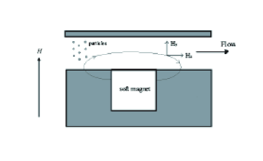
Figure 1: Jian, Zhang and Huang

The microsystem consists of one integrated soft-magnetic elements which is embedded in a nonmagnetic substrate beneath a microfluidic channel as shown in Fig. (1), in which the magnet is $2w$ wide and $2h$ high. The magnetic particles in ferrofluids which pass through the channel can separated according to the different field gradient distribution, and the nonmagnetic particles will be rinsed away. Y axe corresponds to the longitude case mentioned above. Below we will show that when the number of magnetic element increases, the magnetophoresis will become more uniform in both parallel and perpendicular direction to that of particle transport. The bias field $\vec{H}_{\rm bias}$ along y axe and field from the magnet $\vec{H}_{\rm mag}$ which is saturated(saturated magnetization $M_{\rm es}$) when the bias field is added, both contribute to the magnetic field exerted on the particle. Under high frequency of bias field($>10^{3}$Hz), the magnetization of magnet can be viewed constant. Thus the magnetophoretic force is decomposed into two components:

$$F_{\rm mx}=4\pi\mu_{e}R_{\rm eff}^{3}{\rm Re[CMF]}\chi^{{}^{\prime}}[H_{\rm mag,x}\frac{\partial H_{\rm mag,x}}{\partial x}+(H_{\rm mag,y}+H_{\rm bias,y})\frac{\partial H_{\rm mag,y}}{\partial y}],$$ (17)

$$F_{\rm my}=4\pi\mu_{e}R_{\rm eff}^{3}{\rm Re[CMF]}\chi^{{}^{\prime}}[H_{\rm mag,x}\frac{\partial H_{\rm mag,y}}{\partial x}+(H_{\rm mag,y}+H_{\rm bias,y})\frac{\partial H_{\rm mag,x}}{\partial y}].$$ (18)

where $\vec{H}_{\rm mag}$ can be expressed as $H_{\rm mag,x}=\frac{M_{\rm es}}{4\pi}\{{\rm ln}[\frac{(x+w)^{2}+(y-h)^{2}}{(x+w)^{2}+(y+h)^{2}}]-{\rm ln}[\frac{(x-w)^{2}+(y-h)^{2}}{(x-w)^{2}+(y+h)^{2}}]\}$ and $H_{\rm mag,y}=\frac{M_{\rm es}}{2\pi}\{{\rm tan}^{-1}[\frac{2h(x+w)}{(x+w)^{2}+y^{2}-h^{2}}]-{\rm tan}^{-1}[\frac{2h(x-w)}{(x-w)^{2}+y^{2}-h^{2}}]\}$ from  furlani . The magnetophoretic force across the channel can then be be accurately calculated. It could be noted from the equations above that without the bias field magnet-element cannot be magnetized and bias field contributes to the magnetophoretic force, but the bias field itself produce no field gradient in the microchannel. Because the importance of the the contribution from the bias field which causes harmonics of magnetization in the particle, below we will calculate it alone.

III Results

Now we are in the position to study the behavior of magnetophoresis in ferrofluids. Specifically, the external field is set to be $H_{{\rm dc}}=H_{{\rm ac}}=0.01$A/m, high-frequency limit permeability $\mu_{\infty}(0)=8\pi\times 10^{-7}$H/m, dispersion strength $\Delta\mu=32\pi\times 10^{-7}$H/m, medium permeability $\mu_{2}=4\pi\times 10^{-7}$H/m, permanent magnetic moment for each particle $m_{0}=10^{-13}$A/m, characteristic frequency $f_{c}=5\times 10^{3}$Hz, the relaxation time $\tau=5\times 10^{-7}$s, the number density $N=10^{5}$m${}^{-3},$ the length of magnet $w=h=50\mu{\rm m}$, Boltzmann constant $k_{B}=1.38\times 10^{-23}$J/K, the effective radius $R_{\rm eff}=500$nm and the average magnetization of single particle $\alpha=10^{-5}$m^-3.

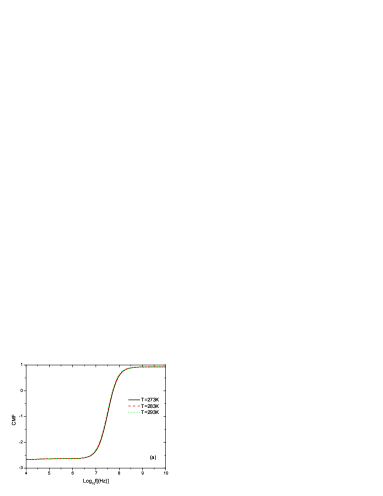
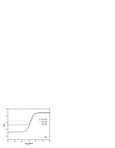
Figure 2: Jian, Zhang and Huang

Figure 2 displays the temperature and anisotropic effect on CMF in magnetophoresis. In Fig. 2(a), it is shown that increasing the temperature T causes slight increase in CMF(about 3$\%$), thus has little effect in magnetophoresis. From Fig. 2(b), the magneophoretic force exhibits strong sensitivity to the anisotropic factor $g_{L}$. When CMF is negative(particles will be repelled from the maximum magnetic gradient), the larger $g_{L}$ is, the smaller repulsion will be. When CMF is positive, with increaseing $g_{L}$ such an attractive force becomes stronger. Furthmore, we predict the anisotropic-dependent crossover frequencies at which there is no net force on the cell particle. The crossover frequency is monotonically increasing function of $g_{L}$, dependent on whether the variation of magnetophoretic force is negative or positive.

Figure 3 and 4 shows the oriental, fundamental, second- and third- order harmonics of the magnetic force $F_{x}$ and $F_{y}$ induced by the bias field mentioned above as a function of the field frequency for various $g_{L}$ in the longitudinal field case. The particle is put in the position x=50nm and y=300nm(see the coordinate in the inset of Fig. 5). The harmonics of magetization of particles will change accordingly as the system alters from isotropic case ($g_{L}=1/3$) to anisotropic ($g_{L}\neq 1/3$) because of the appearance of the particle chains. In detail, stronger anisotropy (namely, decreasing the longitudinal demagnizing factor $g_{L}$) leads to larger magnetic force in the low-frequency region. It can also be observed there is two plateaus in the range 0.03-3MHz and $10^{2}$-$10^{4}$MHz where the magnetic force have slight change and the second and third order harmonics of magnetic force are negligible compared with lower order ones. In fact for the transverse field case, it could be concluded from the sum rule between $g_{L}$ and $g_{T}$ that $g_{L}+2g_{T}=1.$ Because of the coupling between the applied dc and ac magnetic fields, the even-order harmonics are also induced to appear besides the odd-order harmonics for the longitudinal field case, even though only the cubic nonlinearity is considered due to the virtue of symmetry of the system. In addition, the harmonics shown in Figs. 3 and 4 are nonzero at $g_{L}=1/3$ is because of the presence of external fields (i.e., $u_{\rm de}\neq 0$), even though there is no particle interactions (i.e., $u_{\rm mi}=u_{\rm nmi}=0$) as $g_{L}=1/3$, the nonlinear behavior due to the normal saturation could still be induced to occur.

Fig. 5 and 6 displays the magnetic force which is spatially varying across the channel section, when one and two magnets are embedded in the substrate under frequency 10KHz of magnetic field. In Fig. 6 the two magnets are embedded 250$\mu$m away and the $x-y$ coordinate is placed in the midpoint of magnets. Comparing Fig. 5(A) with Fig. 6(A), we find that the force $F_{x}$ for the purpose of separating magnetic particles which is attractive in some regions and repulsive in others along the $x$ axe becomes more uniform, and the force $F_{y}$ has similar nature. In detail the absolute value of magnetic force $F_{x}$ is symmetric in the $x$ direction and become stronger on the edge of the microchannel, while $F_{y}$ is always negative which will repel the particles from the magnets. The uniform separation technique will cause the magnetic particles with different size or permeability become apart into layers in geometry which can in fact not only be used in ferrofluids. The calculation also shows that when more magnets are uniformly embedded, the separation of particles are more efficient. It should be pointed out that the distance between the nearby particles is important to cause spatially uniform magnetic force and it can be chosen for different purpose of separation which may be determined by the capture efficiency for a specific particle sorting or transporting. The time-varying magnetic field can be potentially used for an integrated magnetometer and influences the the viscosity and effective permeability in ferrofluids.

IV Conclusion

We have studied the magnetophoretic particle separation of ferrofluids in microchannel and its nonlinear behavior. The magnetic gradient force is caused by an bias field and the polarized magnets and is found to be spatially uniform in the channel section which can be used for particle selecting or separation. We have derived the equations of nonlinear magnetization of magnetic particles which cause the harmonics of magnetophoresis. The Langevin model and generalized Clausius-Mossotti equation used show how the normal and longitude anomalous anisotropic effect the permeability of ferrofluids, thus the magnetic force. Our analysis demonstrates the viability of using the microchannel system for various bioapplications and other characterization of fluid transporting.

Figure Captions

Fig. 1. (Color online) Schematic graph showing one integrated soft-magnetic elements embeds in a nonmagnetic substrate beneath a microfluidic channel through which ferrofluids flow.

Fig. 2. (a) CMF for different temperatures vs the frequency f of magnetic fields. (b) CMF vs the frequency fof magnetic fields for different anisotropic factors $g_{L}$.

Fig. 3. Oriental, Fundamental, second and third order harmonics of the magnetic force $F_{x}$ vs the field frequency for various $g_{L}$ in the longitudinal field case.

Fig. 4. Same as Fig. 3, but for another force component $F_{y}$.

Fig. 5. (Color online) (A) The spatial magnetic force $F_{x}$ across the channel section, when one magnet embeds in the substrate under frequency 10KHz of magnetic field. (B) The spatial magnetic force $F_{y}$ across the channel section.

Fig. 6. (Color online) Same as Fig. 5, but for two magnets case.

.

.

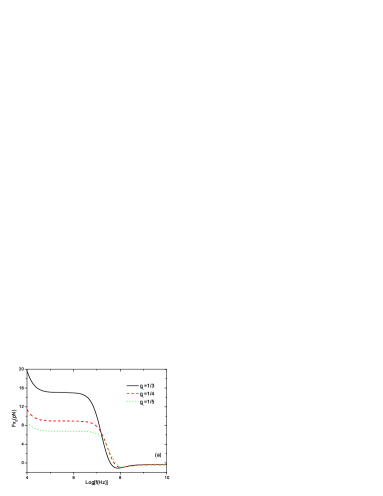
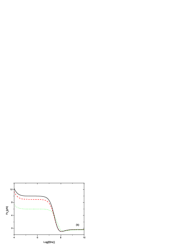
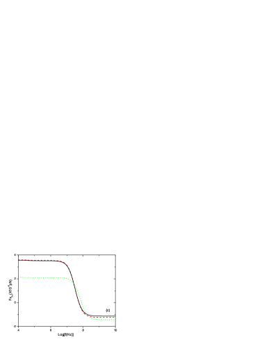
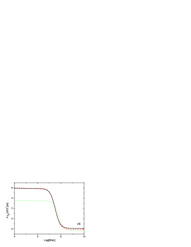
Figure 3: Jian, Zhang and Huang

.

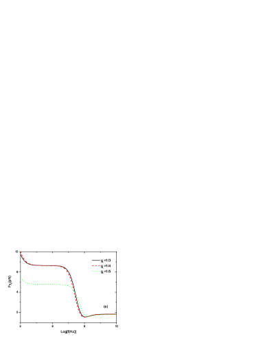
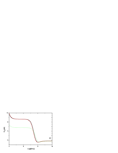
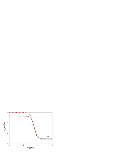
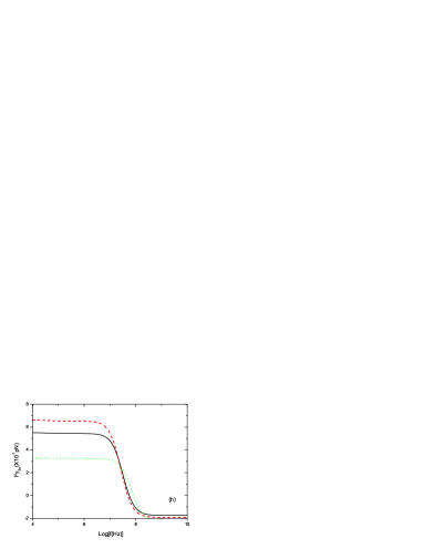
Figure 4: Jian, Zhang and Huang

.

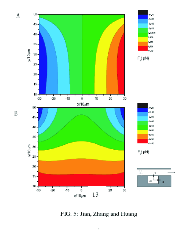
Figure 5: Jian, Zhang and Huang

.

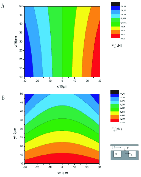
Figure 6: Jian, Zhang and Huang

.

References

- (1) E. Verpoorte and N. F. De Rooij, Proc. IEEE 91, 930 (2003).
- (2) E. P. Furlani, Jour. Appl. Phys. 99, 024912 (2006) and the references therein of the particle transport in the microsystem.
- (3) E. L. Bizdoaca, M. Spasova, M. Farle, M. Hilgendorff, L. M. Liz-marzan and F. Caruso, J. Vac. Sci. Technol. A 21(4), 1515 (2003).
- (4) Ki-Ho Han and A. Bruno Fraziera, Jour. Appl. Phys. 96, 5797 (2004).
- (5) F. Paul, S. Roath, D. Melville, D. C. Warhurst and J. O. S. Osisanya, Lancet. 2, 70 (1981).
- (6) J. W. Choi, K. W. Oh, J. H. Thomas, W. R. Heineman, H. B. Halsall, J. H. Nevin, A. J. Helmicki, H. T. Henderson, and C. H. Ahn, Lab Chip. 2, 27 (2002).
- (7) D. W. Inglis, R. Riehn, J. C. Sturm and R. H. Austin, Jour. Appl. Phys. 99, 08K101 (2006).
- (8) A. T. Skjeltorp, Phys. Rev. Lett. 51, 2306 (1983); R. R. Birss, R. Gerber, and M. R. Parker, IEEE Trans. Magn. MAG-12, 892 (1976).
- (9) G. Wang and J. P. Huang, Chem. Phys. Lett.421, 544 (2006); J. P. Huang and K. W. Yu, Jour. Chem. Phys. 121, 7526 (2004).
- (10) J. Zhang, C. Boyd and W. Luo, Phys. Rev. Lett. 77, 390 (1996).
- (11) O. Ayala Valenzuela, J. Matutes Aquino, R. Betancourt Galindo, O. Rodrguez Fernndez, P. C. Fannin, A. T. Giannitsis. J. Appl. Phys. 97, 10Q914 (2005).
- (12) K. H. Bennemann, Nonlinear Optics in Metals, (Clarendon Press, Oxford, 1998).
- (13) D. Frhlich, S. Leute, V. V. Pavlov, R. V. Pisarev. Phys. Rev Lett. 81, 3239 (1998).
- (14) Y. Ogawa, Y. Kaneko, J. P. He, X. Z. Yu, T. Arima and Y. Tokura. Phys. Rev Lett. 92, 047401 (2004).
- (15) C. J. F. Bttcher, third edn. Theory of Electric Polarization, vol. 1, Elsevier, Amsterdam (1993).
- (16) O. Levy, D. J. Bergman and D. Stroud, Phys. Rev. E. 52, 3184 (1995).
- (17) C. K. Lo and K. W. Yu, Phys. Rev. E 64, 031501 (2001).
- (18) L. D. Landau, E. M. Lifshitz, and L. P. Pitaevskii, Electrodynamics of Continuous Media, 2nd ed. (Pergamon press, New York, 1984), Chap. II.
- (19) J. E. Martin, R. A. Anderson, and C. P. Tigges, J. Chem. Phys. 108, 3765 (1998); J. E. Martin, R. A. Anderson, and C. P. Tigges, J. Chem. Phys. 108, 7887 (1998).
- (20) M. I. Shliomis, Sov. Phys.-Usp. 17, 53 (1974)
- (21) H. Frhlich, Theory of Dielectrics, (Oxford University Press, London, 1958)
- (22) C. L. Asbury and Ger van den Engh, Biophys. Jour. 74, 1024 (1998)
- (23) Chin-Yih Hong, C. C. Wu, Y. C. Chiu, S. Y. Yang, H. E. Hornga, and H. C. Yang, Appl. Phys. Lett. 88, 212512 (2006)
- (24) T. B. Jones, Electromechanics of Particles (Cambridge University Press, Cambridge, 1995), Chap.III.