Integral estimator of broadband omnidirectionality

Abstract

By using the notion of wavelength- and angle-averaged reflectance, we assess in a systematic way the performance of finite omnidirectional reflectors. We put forward how this concept can be employed to optimize omnidirectional capabilities. We also apply it to give an alternate meaningful characterization of the bandwidth of these systems.

Floquet-Bloch theory warrants that the behavior of periodically stratified media is determined by the trace of the transfer matrix of the basic period. Indeed, whenever the magnitude of this trace is greater than 2, no waves propagate in the structure and then a stop band appears.

In the context of electromagnetic optics, this notion is at the basis of photonic crystals Dowling (that is, one-dimensional periodic layered structures), which have been attracting a lot of attention because of their amazing property of acting as omnidirectional reflectors (ODRs): they reflect light at any polarization, any incidence angle, and over a wide range of wavelengths Yablonovitch1987 ; John1987 ; Fink1998 ; Dowling1998 ; Chigrin1999 .

Although there are a number of approaches for ensuring a trace greater than 2 in the basic period Liu1997 ; Macia1998 ; Cojocaru2001 ; Lusk2001 ; Peng2002 , the most feasible design involves two materials with refractive indices as different as possible. Such a bilayer system is usually designed at quarter-wave thickness (at normal incidence), which is enough to guarantee ODR Southwell1999 ; Chigrin1999a ; Lekner2000 . However, this assumes perfect periodicity and so requires the system to be strictly infinite. Of course, this is unattainable in practice and one is led to consider stacks of $N$ periods, which are often appropriately called finite periodic structures Lekner1994 . One can rightly argue that when $N$ is high enough (say, 50 or more), there should be no noticeable differences with the ideal infinite case Lusk2005 . But there are commercial ODR designs considering only very few periods ssp and, in such a situation, the optimization of the basic period deserves a careful and in-depth study.

To shed light on this issue it is essential to quantify the ODR performance in a manner that permits unambiguous comparison between different structures. We hold to previous suggestions Yonte2004 ; Barriuso2005 , but to take into due consideration the key role of the bandwidth, we propose here to average the reflectance over all the incidence angles and all the wavelengths in the spectral range. With this tool at hand, we revisit finite ODRs and characterize their properties, addressing, as a side product, a proper picture of the omnidirectional bandwidth for these systems.

We begin by briefly recalling some background concepts. The basic period of the finite ODR consists of a double layer made of materials with refractive indices $(n_{L},n_{H})$ and thicknesses $(d_{L},d_{H})$, respectively. The material $L$ has a low refractive index, while $H$ is of a high refractive index. To characterize the optical response we employ the transfer matrix, which can be computed as $\mathsf{M}=\mathsf{M}_{L}\,\mathsf{M}_{H}$, where $\mathsf{M}_{L}$ and $\mathsf{M}_{H}$ are the transfer matrices of each layer, whose standard form can be found in any textbook Yeh1988 .

As we have mentioned before, band gaps appear whenever the trace of the basic period satisfies

$$|\mathop{\mathrm{Tr}}\nolimits(\mathsf{M})|\geq 2\,.$$ (1)

This condition should be worked out for both basic polarizations. However, it is known that whenever Eq. (1) is fulfilled for $p$ polarization, it is always true also for $s$ polarization. The $p$-polarization bands are more stringent than the corresponding $s$-polarization ones Lekner1987 and we thus restrict our study to the former.

We next consider an $N$-period structure whose basic cell is precisely the bilayer $LH$. We denote this as $[LH]^{N}$ and its overall transfer matrix is simply $\mathsf{M}^{N},$ from which calculating its reflectance $\mathcal{R}^{(N)}$ is straightforward. According to our previous discussion, we average over all the incidence angles and all the wavelengths in the spectral interval $\Delta\lambda=\lambda_{\mathrm{max}}-\lambda_{\mathrm{min}}$ of interest

$$\overline{\mathcal{R}}^{(N)}=\frac{1}{\Delta\lambda}\int_{\lambda_{\mathrm{min}}}^{\lambda_{\mathrm{max}}}\left(\frac{2}{\pi}\int_{0}^{\pi/2}\mathcal{R}^{(N)}\ d\theta\right)d\lambda\,,$$ (2)

and take this as an appropriate figure of merit to assess the performance as an ODR. Once the materials have been chosen, $\overline{\mathcal{R}}^{(N)}$ is a function exclusively of the layer thicknesses.

As a case study, we take the materials to be cryolite (Na₃AlF₆) and zinc selenide (ZnSe), with refractive indices $n_{L}=1.34$ and $n_{H}=2.568$, respectively, at the wavelength $\lambda=0.65\ \mu$m. The spectral window considered is from $\lambda_{\mathrm{min}}=0.5\ \mu$m to $\lambda_{\mathrm{max}}=0.8\ \mu$m. In this range, the refractive index of the cryolite can be considered, to a good approximation, as constant, while for the zinc selenide we use the Sellmeier dispersion equation $n_{H}^{2}(\lambda)=4+1.9\lambda^{2}/[\lambda^{2}-(0.336)^{2}]$, where $\lambda$ is expressed in microns.

Many commercial packages are available to perform layer optimization. In the case of ODR, common methods optimize a merit function that (quadratically) measures how the calculated reflectance separates from unity (ideal target) at some definite angles and at some definite wavelengths. For example, TFCALC uses needle optimization to find the best thicknesses for such a merit function. We have preferred, however, to implement a gradient-based modified quasi-Newton algorithm (using the Fortran NAG libraries), for its consistency with the problem investigated, which is continuous.

Figure 1: (Color on line) Averaged reflectance $\overline{\mathcal{R}}^{(N)}$ in terms of number of periods for the optimized $[LH]^{N}$ systems (blue triangles) and for the same system when all the thicknesses can be different (red circles). Solid lines represent the fittings to these points.

We have optimized the system $[LH]^{N}$ for $N$ running from 5 to 20. When the thicknesses are kept equal by pairs, so as the structure retains its periodicity, we find thicknesses distributed around $d_{L}\simeq 145$ nm and $d_{H}\simeq 60$ nm. The variation of $\overline{\mathcal{R}}^{(N)}$ with $N$ is shown in Fig. 1, and can be numerically fitted to $\overline{\mathcal{R}}^{(N)}=0.774+0.365\times 10^{-3}\ N$; i.e., a linear dependence with an extremely small slope. We have also worked out the instance when all the thicknesses may vary independently (though now the system is not strictly periodic). The optimum thicknesses oscillate a lot, without a definite pattern (we do not list all of these values because of space limitation). However, as is clear from Fig. 1, $\overline{\mathcal{R}}^{(N)}$ shows an exponential increasing that can be suitably represented by $\overline{\mathcal{R}}^{(N)}=0.625+0.369[1-\exp(-0.132N)]$.

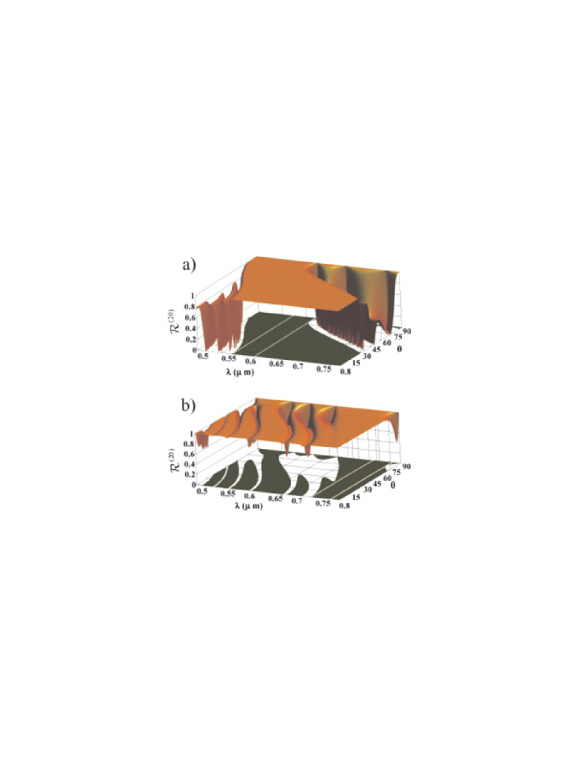
Figure 2: (Color on line) Plot of the reflectance $\mathcal{R}^{(20)}$ as a function of the incidence angle $\theta$ (in degrees) and the wavelength $\lambda$ (in $\mu$m). In a) we have the $[LH]^{20}$ system, while in b) the thicknesses are allowed to be different. At the bottom plane, we show the contour plots corresponding to a reflectance 0.99. The white lines delimit the zones in which this reflectance is greater than 0.99 for all the angles of incidence.

To gain further insights into these striking differences, in Fig. 2 we have plotted the reflectance $\mathcal{R}^{(20)}$ for the optimum thicknesses rep corresponding to $N=20$ as a function of the angle of incidence $\theta$ and the wavelength $\lambda$. At the bottom plane we have also included the contours of the regions where this reflectance is greater than 0.99. While for the $[LH]^{20}$ system, the top zone looks quite flat and very close to unity, the dips are very deep indeed. On the contrary, when we allow for different thicknesses, the top zone presents small ripples, but the dips are much less pronounced. Curiously enough, the $[LH]^{20}$ system gives a wider region lying above the 0.99 level. We have also marked two stripes (within parallel lines) in which the reflectance is greater than 0.99 for all the angles of incidence (and that, roughly speaking, could be identified with stop bands). Although of similar extension, they lie in quite different spectral ranges. We have repeated these calculations with other values of $N$, observing essentially the same kind of behavior.

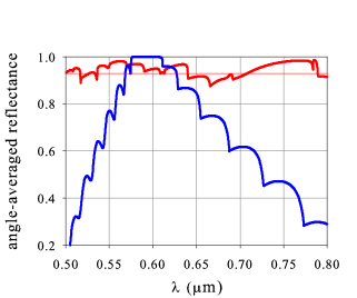
Figure 3: (Color on line) Angle-averaged reflectance in terms of the wavelength $\lambda$ for the optimized $[LH]^{20}$ system (blue) and for the analogous system with different thicknesses (red). The line of reflectance equal to 0.95 is also shown.

To proceed further, in Fig. 3 we have represented the angle-averaged reflectance [i.e., the magnitude in parentheses in Eq. (2)] for the same two systems as in Fig. 2, in terms of the wavelength $\lambda$. Obviously, the area under the curve is precisely $\overline{\mathcal{R}}^{(20)}$. It is clear that for different thicknesses, this area is considerably bigger (so, it is really an optimum), while the $[LH]^{20}$ is better behaved in a narrow range going from 0.57 $\mu$m to around 0.62 $\mu$m (which matches well with the stop band shown in Fig. 2.a). In other words, the optimum system remarkably improves the behavior in the spectral wings, while it little affects (or even deteriorates) the behavior in the “good” central region. The ripples in both curves are caused by the dips appearing in Fig. 2 for each line of $\lambda$ constant.

In this respect, we wish to note that, in our opinion, the notion of bandwidth becomes fuzzy for ODRs. Usually Yeh1988 , it is defined as $\delta\lambda=\lambda_{+}-\lambda_{-}$ [and sometimes Southwell1999 normalized to the central wavelength $(\lambda_{+}+\lambda_{-})/2$], where $\lambda_{+}$ and $\lambda_{-}$ are the longer- and shorter-wavelength edges for given ODR bands [i.e., the two solutions of Eq. (1)]. This is meaningful in the limit $N\rightarrow\infty$, when these band edges make unambiguous sense, but fails for our more realistic situation. Other authors Orfanidis2004 note that the common reflecting band for both polarizations and for angles up to a given $\theta_{\mathrm{M}}$ (which is defined by convention) is $[\lambda_{-}(\theta_{\mathrm{M}}),\lambda_{+}(0)]$ and the corresponding bandwidth $\delta\lambda=\lambda_{+}(0)-\lambda_{-}(\theta_{\mathrm{M}})$. Again, this kind of definition assumes the existence of a full band, which is only true for the strictly periodic case.

We emphasize that all the relevant information about omnidirectionality is contained in the angle-averaged reflectance. Furthermore, being an integral estimator, it does not rely on the values of the reflectance at some specific relevant angles. For this reason, a sensible choice for defining the bandwidth is precisely the spectral range(s) for which this angle-averaged reflectance is bigger than a fixed threshold value. For example, if we set this value to, say 0.95, it is evident in Fig. 3 that the bandwidth for the $[LH]^{20}$ system is always poor.

To sum up in a few words, we have exploited the notion of wavelength- and angle-averaged reflectance to explore in a systematic way the performance of finite ODRs. Needless to say, our approach is general and can be applied to other materials and other spectral regions.

This work has been supported by the Spanish Research Agency Grant FIS2005-06714.

References

- (1) A complete and up-to-date bibliography on the subject can be found at http://baton.phys.lsu.edu/~jdowling/pbgbib.html.
- (2) E. Yablonovitch, Phys. Rev. Lett. 58, 2059–2062 (1987).
- (3) S. John, Phys. Rev. Lett. 58, 2468–2469 (1987).
- (4) Y. Fink, J. N. Winn, S. Fan, C. Chen, J. Michel, J. D. Joannopoulos, and E. L. Thomas, Science 282, 1679–1682 (1998).
- (5) J. P. Dowling, Science 282, 1841–1842 (1998).
- (6) D. N. Chigrin, A. V. Lavrinenko, D. A. Yarotsky, and S. V. Gaponenko, Appl. Phys. A 68, 25–28 (1999).
- (7) N. H. Liu, Phys. Rev. B 55, 3543–3547 (1997).
- (8) E. Maciá, Appl. Phys. Lett. 73, 3330–3332 (1998).
- (9) E. Cojocaru, Appl. Opt. 40, 6319–6326 (2001).
- (10) D. Lusk, I. Abdulhalim, and F. Placido, Opt. Commun. 198, 273–279 (2001).
- (11) R. W. Peng, X. Q. Huang, F. Qiu, M. Wang, A. Hu, S. S. Jiang, and M. Mazzer, Appl. Phys. Lett. 80, 3063–3065 (2002).
- (12) W. H. Southwell Appl. Opt. 38, 5464–5467 (1999).
- (13) D. N. Chigrin, A. V. Lavrinenko, D. A. Yarotsky, and S. V. Gaponenko, J. Lightw. Technol. 17, 2018–2024 (1999).
- (14) J. Lekner, J. Opt. A 2, 349–353 (2000).
- (15) J. Lekner, J. Opt. Soc. Am. A 11, 2892–2899 (1994).
- (16) D. Lusk and F. Placido, Thin Solid Films 492, 226–231 (2005).
- (17) http://www.sspectra.com/designs/omnirefl.html
- (18) T. Yonte, J. J. Monzón, A. Felipe, and L. L. Sánchez-Soto, J. Opt. A 6, 127–131 (2004).
- (19) A. G. Barriuso, J. J. Monzón, L. L. Sánchez-Soto, and A. Felipe, Opt. Express 13, 3913–3920 (2005).
- (20) P. Yeh, Optical Waves in Layered Media (Wiley, New York, 1988).
- (21) J. Lekner, Theory of Reflection (Kluwer Academic, Dordrecht, 1987).
- (22) To ensure the reproducibility of our results, we quote here the optimum thicknesses (expressed in nm). For the they are and . When all of them are different, we have for the -medium: 190, 111, 184, 99, 164, 145, 173, 180, 118, 132, 143, 134, 193, 101, 155, 122, 100, 165, 91, 110. For the medium they are 58, 141, 92, 140, 54, 122, 88, 71, 79, 46, 47, 72, 125, 143, 87, 112, 106, 59, 120, 116.
- (23) S. J. Orfanidis, Electromagnetic Waves and Antennas. (http://www.ece.rutgers.edu/orfanidi/ewa/). Chap. 7.