A novel shear flow instability triggered by a chemical reaction in the absence of inertia

Abstract

We present an experimental investigation of a novel low Reynolds number shear flow instability triggered by a chemical reaction. An acid-base reaction taking place at the interface between a Newtonian fluid and Carbopol-$940$ solution leads to a strong viscosity stratification, which locally destabilizes the flow. Our experimental observations are made in the context of a miscible displacement flow, for which the flow instability promotes local mixing and subsequently improves the displacement efficiency. The experimental study is complemented by a simplified normal mode analysis to shed light on the origin of the instability.

I Introduction

Designing a method to locally control the hydrodynamic stability of a shear flow is of importance in many practical and laboratory applications. In the absence of inertia, non-equilibrium hydrodynamical systems may lose stability if a relevant physical field becomes stratified. To help illustrate this point, convective motion may be induced in a thin static layer of fluid when heated from below convection or gravity induced density stratification may sustain internal gravity waves, Landau . An alternative method of locally destabilizing low Reynolds number ($\mathrm{Re}$) shear flow would be to induce significant changes in the local fluid rheology. Although flows with a strongly stratified viscosity have been proved to be theoretically unstable, Ern03 this situation has never been demonstrated experimentally. With flows of simple Newtonian fluids, it is difficult to vary the viscosity locally to induce an instability. With complex (or structured) fluids ,however, the situation is significantly different: the rheology is strongly coupled to the molecular scale organization of the fluid. This opens a new possibility of locally controlling the viscosity by inducing local changes in the molecular structure via a chemical reaction. The advantage of such method is that a chemical reaction may be controlled by either mass transfer or by local heating or cooling. In this paper we show experimentally that a displacement flow of two miscible liquids may be destabilized by local changes in the fluid rheology triggered by an acid-base reaction at their interface.

Miscible displacements have been studied in depth within the context of Hele-Shaw and porous media displacement instabilities, initially motivated by a desire to better understand oil reservoir recovery issues, e.g. Tan86 ; Hick86 ; Chan86 ; Yort87 ; Tan88 ; Yort88 , and this science is now well developed. In the Navier-Stokes setting, miscible displacements through small ducts have been studied both experimentally and numerically, Peti96 ; Chen96 ; Rako97 ; Yang97 . For the large Péclet number ($\mathrm{Pe}$) regime, depending on the viscosity ratio $m$, quasi-steady viscous fingers may form and propagate with a sharp displacement front that is retained over long timescales. The efficiency of the displacement (defined as the amount of fluid removed from the pipe walls) may be either measured or estimated using computation or asymptotic methods, see e.g. Yang97 ; Laje99a . In the case that the fingers remain stable, the residual wall layers thin at a rate that is significantly slower than the mean flow and the efficiency of the displacement is $<1$. Although asymptotically the efficiency may approach $1$ as $t\to\infty$, for various practical reasons one might not want to wait.

To improve the displacement efficiency, one method would be to trigger a flow instability, such that the perturbed interface disturbs the residual wall layers. At large $\mathrm{Re}$, multi-layer flows of viscous fluids are usually unstable, but linear interfacial instabilities are also found for quite low $\mathrm{Re}$. Dating from the late 1960’s, there are a number of studies involving both immiscible and miscible fluids, e.g. Yih67 ; Hick71 . An extensive review can be found in the text Jose93 , and the physical mechanisms governing short and long wavelength instabilities have been explained by Hinc84 ; Char00 . These studies generally refer to the situation where there is a jump in the viscosity at the interface between two fluids. If the change in viscosity is instead gradual, e.g. due to a diffuse interfacial region, then the stability characteristics appear to mimic those of the system with the viscosity jump, see Ern03 .

In porous media, non-monotone viscosity variations are known to cause linear instability of planar displacements, see Hick86 ; Chik88 ; Mani93 , as can be predicted by classical mobility ratio arguments. Here however, we are in the Navier-Stokes regime and consider primarily shear flows. Also we have sharp localized change in viscosity, which is hard to achieve in “simple” fluids, where viscosity is often related to slowly varying concentration or temperature, i.e. due to molecular structure of the fluid. For complex (or structured) fluids the viscosity depends strongly on the microscopic structure. In the case of polymer solutions, the microscopic structure of the fluid can be locally modified by either mechanical means (e.g. shear-thinning, Bird ) or chemical means, by locally modifying the chemical bonds between neighboring polymer molecules.

In recent years there have been a number of studies of systems with coupled chemical reactions and fluid flow, so it is natural to examine the relation to this literature. In the first place even without fluid flow, spatially traveling waves can be observed in chemically excitable media governed by coupled reaction-diffusion systems, see e.g. the review Tyso88 . These fronts may frequently destabilize linearly. There is often coupling between the reactions, and hence a mechanism of feedback, and sometimes a significant difference in the reaction rate constants. Slightly simpler systems involve single species auto-catalytic reactions, which mathematically admit traveling (chemical) wave solutions. Systems in which the auto-catalytic reaction results in a significant density change have been studied intensively. The base traveling chemical wave is coupled with a Rayleigh-Taylor problem. There are consequently a wide range of stable and unstable situations to be studied, and even more once a base fluid velocity is considered. A selection of the many works includes Pojman90 ; Edwards91 ; Vasquez91 ; Vasquez94 ; Edwards02 ; Vasquez04 ; Hern06 ; Lima06 . Of closer relation to our work is the sequence of papers, DeWit97a ; DeWit97b ; DeWit99a ; DeWit99b , which have considered a concentration dependent viscosity in the context of miscible porous media displacements. Although interesting and a useful guide in methodology, direct relevance of these many papers to our study is in fact limited. Our system is not auto-catalytic, there are no buoyancy effects and the displacement flow is not a gradient flow.

I.1 Industrial motivation

The motivation for our study comes from the construction of oil and gas wells. Since the early 1990’s there has been an increasing number of wells that are constructed with long horizontal sections. The worlds longest extended reach wells have horizontal sections in the $10-15$ km range, but these are exceptional. More routinely, wells are built with horizontal extensions of up to $\sim 7$ km. One of the key barriers in constructing longer wells comes from simple hydraulic friction. In a vertical well, both the pore pressure of reservoir fluids and the fracture pressure of the reservoir rock increase with depth, approximately linearly. Judicious choice of fluid density and circulating flow rates keeps the wellbore pressure inside the so-called “pore-frac envelope”, i.e. the region where the porous rock does not fracture. In a horizontal well section, the pore-frac envelope is unchanged with length along the well, but the frictional pressure increases with length, leading to eventual breaching of the envelope Bourg ; Porefrac ; Horiz .

There is a consequent interest in methods and fluids that control the frictional pressure in some way. Two operations where this is important are drilling and cementing. In the cementing process, Nels90 , it is necessary to displace the drilling mud with a spacer fluid and then with a cement slurry. As the section is horizontal, density differences between the fluids lead to stratification and should be avoided. Instead the focus is on controlling the rheology of the fluids and the displacement flow itself. The idea behind the reactive instability that we are studying is explained by the following simple calculation.

Suppose simplistically that we have Newtonian fluids, a circular pipe of radius $\hat{R}$ and that we wish to displace at mean speed $\hat{U}_{0}$. If $\Delta\hat{p}_{e}$ is the difference between pore and fracture limits, then we are restricted to a length-viscosity combination:

$$8\frac{\hat{L}\hat{\eta}\hat{U}_{0}}{\hat{R}^{2}}<\Delta\hat{p}_{e}.$$

Normally, we will need to select the viscosity of the spacer fluid, $\hat{\eta}_{s}>m\hat{\eta}_{d}$, where $m>1$ and $\hat{\eta}_{d}$ is the viscosity of the in-situ fluid, e.g. drilling mud, so that

$$\hat{L}<\frac{\hat{R}^{2}\Delta\hat{p}_{e}}{8m\hat{\eta}_{d}\hat{U}_{0}}.$$ (1)

Suppose instead we are able to pump a spacer fluid of viscosity $\hat{\eta}_{s}\leq\hat{\eta}_{d}$, that reacts with the in-situ fluid to cause a local instability. If the instability causes effective mixing across the pipe after the fluid has traveled $k$ radii, we may model this process by a radial diffusivity $\hat{D}_{r}\sim(\hat{R}\hat{U}_{0})/k$. Provided $k\ll\hat{L}/\hat{R}$, we have an effective Taylor dispersion process in which the mixed zone diffuses axially along the pipe, relative to the mean flow. This axial diffusion of the mixed region is governed by a dispersion coefficient of order $\sim kD_{T}(\hat{R}\hat{U}_{0})$, where $D_{T}=1/48$ is the Taylor dispersion coefficient for a pipe. After traveling a distance $\hat{L}$, the mixed zone will have dispersed axially a distance

$$\hat{L}_{\mathrm{mix}}\sim\left[kD_{T}\hat{R}\hat{L}\right]^{1/2}.$$

If the reacted mixture has viscosity $(a+1)\hat{\eta}_{s}$, where $a\geq 0$, then the frictional pressure drop along the pipe can be limited by

$$\Delta\hat{p}_{e}>8\frac{\hat{\eta}_{s}\hat{U}_{0}}{\hat{R}^{2}}\left(\hat{L}+a\hat{L}_{\mathrm{mix}}\right),$$

and the pipe length restriction is

$$\hat{L}<\frac{\hat{R}^{2}\Delta\hat{p}_{e}}{8\hat{\eta}_{s}\hat{U}_{0}(1+a[kD_{T}\hat{R}/\hat{L}]^{1/2})}.$$ (2)

Therefore, for a given pore-frac limit, we may increase the length of the well that may be effectively displaced provided that:

$$\frac{m\hat{\eta}_{d}}{\hat{\eta}_{s}(1+a[kD_{T}\hat{R}/\hat{L}]^{1/2})}>1.$$ (3)

Over lengths sufficiently long that $a[kD_{T}\hat{R}/\hat{L}]^{1/2}\ll 1$, we achieve a length increase by a modest factor $m\hat{\eta}_{d}/\hat{\eta}_{s}$.

Even modest increases in length may have a large impact, both economically and environmentally. In modern offshore drilling, one vertical well drilled down from the seabed may act as the stem for many lateral horizontal branches, extending radially outwards. Thus, increases in the length of horizontal branches correspond to (length)² increases in the area of reservoir that may be reached and contribute to a reduction in the number of wellheads required. This reduces the cost of the field development reduces the environmental footprint, lessens risks of leakage of reservoir fluids and eventually makes for an easier well abandonment.

I.2 Organization

Our paper is organized as follows. Section II describes the experimental setup, the measurement techniques and the rheology of our fluids. Experimental results are presented in §III. Section IV introduces a simple hydrodynamic stability model that gives insight into the instabilities we observe. The paper closes with a brief discussion of our findings and a discussion on future theoretical and experimental studies.

II Description of the experiments

II.1 Experimental apparatus and techniques

All experiments were conducted in the apparatus illustrated schematically in Fig. 1. It consists of a horizontal flow channel FC with circular cross section of radius $\hat{R}=5.5$ mm and length $\hat{L}=1.2$ m, immersed in a water filled glass container GC to ensure distortion-free flow illumination and imaging. The system was illuminated by a thin laser sheet passing horizontally through the transparent walls of both the glass container and the flow channel, at the middle vertical position. The laser sheet has a thickness of approximately $50~{}\mu$m in the center of the set-up and about $160~{}\mu$m near the walls of the channel. It was generated by passing a laser beam delivered by a $150$ mW solid state laser, L, through a block of two crossed cylindrical lenses, CO, mounted in a telescopic arrangement.

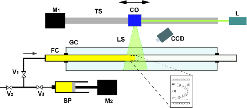
Figure 1: Schematic view of the experimental apparatus: FC-flow channel, GC-glass container, L-solid state laser, CO-cylindrical optics, LS-laser sheet, CCD -camera, $\mathbf{M_{1,2}}$-stepping motors, $\mathbf{V_{1,2,3}}$-valves, TS-horizontal translational stage, SP-syringe pump. The lower inset illustrates schematically the flow configuration: the full curve represents the interface between fluids, the dotted lines indicate the reacting region and the horizontal arrows point the mean flow direction.

The flow was imaged from the top (Fig. 1) with a charge coupled device camera, CCD, equipped with a $35$ mm photographic lens. The images were digitized with $8$ bit quantization and $640\times 760$ pixels resolution (which accounts for $130~{}\mu$m). The size of the imaged area was thus $1.4\times 1.4~{}\mathrm{cm}^{2}$.

The flow in the channel was induced by a syringe pump SP actuated by a precise stepping motor, $\mathbf{M_{1}}$ (from $CBVL$, Vancouver) and controlled by computer via a serial port. The inflow mean velocity was controlled with an accuracy better than $100~{}\mu$m/s. In order to monitor the evolution of the fluid interface downstream, the CCD and the cylindrical optics block, CO, were mounted on a linear translational stage parallel to the flow channel (TS in Fig. 1). The stage was actuated by a stepping motor $\mathbf{M_{1}}$ and controlled by computer via a serial port. The typical configuration of fluids during the horizontal displacement experiments is schematically illustrated in the inset of Fig. 1.

The stability of the interface between fluids was investigated using either Laser Induced Fluorescence ($LIF$), or Digital Particle Image Velocimetry ($DPIV$). The image acquisition software was developed in-house and allowed us to adjust the time delay between successive frames in relation to the local flow velocity (in order to keep the mean particle displacement in the range $5-30$ pixels). For low values of the flow velocity the time delay was $66$ ms. For higher flow speeds, the delay was decreased to $16$ ms. The fluids were seeded with either a small amount (approx. $160$ ppm) of $20~{}\mu$m Polyamide spheres (from Dantec Inc.) for $DPIV$ measurements, or with fluorescein sodium salt (Sigma Aldrich) for the $LIF$ measurements. Time series of the velocity fields were obtained by a multi-pass $DPIV$ algorithm Scarano . The spatial resolution was $167~{}\mu$m. The accuracy of the method has been carefully checked by running test measurements for low Reynolds number Poiseuille flows with Newtonian fluids and comparing then with the analytical solution.

In addition to these techniques, we have developed a third visualization method to measure the local pH in the flow field. We do so by using a $pH$ sensitive colored dye, Bromothymol Blue (Sigma Aldrich). The local value of the $pH$ near the interface was assessed by measurements of the color distribution in the field of view. With this we are able to estimate the local rheological properties.

II.2 Fluid properties

We have used the same base fluids for all our experiments, with various adjustments to the levels of acid and base used in each fluid to examine different regimes. The displacing fluid, Fluid $1$, was a $65\%$ aqueous sucrose solution. The pH of this fluid was varied between $7$ and $11$ by titration with different amounts of $NaOH$ ranging from $150$ parts per million ($ppm$) and $~{}300~{}ppm$. The displaced fluid, Fluid $2$, was a mixture of a 5% (wt) Carbopol 940 (C-940) solution and a $65\%$ (wt) sucrose solution in deionized water. C-940 is generally referred to as a weak polyacrylic acid and dissociates in solution. The $pH$ of this solution is typically between two and three. During our experiments, neutralization of C-940 molecules present in Fluid $2$ occurs locally, in the vicinity of the interface,through contact with Fluid $1$.

The $pH$ of the fluids were measured with a thermally corrected digital $pH$ meter (Topac Instruments) with $1.5\%$ accuracy. The rheological properties of both fluids $1$ and $2$ were measured with a stress controlled rotational rheometer: $CVOR$ acquired from Bohlin Instruments (Malvern Inc., www.malvern.co.uk). Example flow curves at $22^{\circ}C$ of Fluid $1$, Fluid $2$ (at $pH\approx 3$) and Fluid $2$ (at $pH\approx 7$), are presented in Fig. 2. As shown, the viscosity of Fluid $1$ is independent of shear rate. With Fluid $2$ at a $pH\approx 3.2$, the viscosity is also approximately constant. As a guide, at a shear rate of 2 $s^{-1}$ we have viscosities $\hat{\eta}_{1}=114$ mPas and $\hat{\eta}_{2}=138$ mPas, for fluids $1$ and $2$ respectively. As the $pH$ is increased the rheology of Fluid $2$ changes dramatically (see Fig. 2). A detailed study of the coupling between the $pH$, the molecular structure and the rheological properties of C-940 has been recently reported in Frisken .

In order to quantify the dependence of the rheological properties of Fluid $2$ on the $pH$, several batches have been prepared at different $pH$ values, and the rheological tests have been conducted. The $pH$ dependence of the shear viscosity of fluid $2$ at rate of strain $\dot{\gamma}=2~{}s^{-1}$, is shown in Fig. 3a. In the range of $pH$ shown, the shear viscosity increases monotonically, up to a value nearly two orders of magnitude larger than the non-neutralized value. The $pH$ dependence of the measured yield stress of Fluid $2$ is shown in Fig. 3b. A further increase of the $pH$ (data not shown in Fig. 3) results in destruction of the gel structure, which causes both viscosity and yield stress to drop to their initial low $pH$ values.

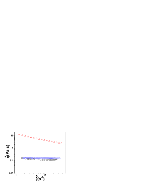
Figure 2: Shear rate dependence of the viscosities of the fluids: ($\circ$) displaced fluid 2 with $pH\approx 3$, ($\Box$) displacing Fluid 1 , ($\triangle$) displaced Fluid 2 with $pH\approx 7$.

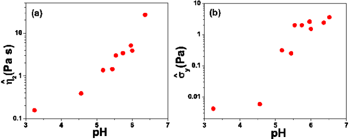
Figure 3: Dependence of the rheological properties of fluid $2$ on $pH$: (a) viscosity measured at $\dot{\gamma}=2s^{-1}$ (b) yield stress.

II.3 Experimental procedure

Our displacement experiments were conducted as follows. First, the alignment of the laser sheet and focus of the camera is carefully checked at several locations downstream. Second, the valves $V_{1}$, $V_{2}$ are open and the channel is initially filled with Fluid $2$. Next, we close valve $V_{1}$, open valve $V_{3}$ and start to drive the syringe pump at very low speeds for several tens of seconds. This procedure allows us to eliminate any air bubbles generated during the filling of the flow channel. Finally, we close valve $V_{2}$ and open valves $V_{1}$ , and set the fluids in motion by operating the syringe pump at the desired speed. The flow images were usually acquired halfway down length of the pipe, though in some of the experiments the camera and the laser sheet were moved at constant speed along the flow channel. Approximately $1000$ flow images were acquired both before the entrance of the fluid interface in the measuring window and after. Details of the experimental conditions tested are given in Table 1.

III Experimental results

We propose to control the stability of an interface between a Newtonian and a C-940 solution by inducing changes in the local fluid rheology via an acid-base reaction, which depends on the free charge mismatch across the interface,and the $pH$ of each fluid. With $1\%$ NaOH, the saccharose solution (Fluid 1) has a pH around $11$. When in contact with Fluid $2$ at $pH\approx 3$, neutralization occurs near the interface resulting in a thin layer of high viscosity fluid, see Fig. 2. The high viscosity interfacial layer apparently undergoes a self-sustained hydrodynamic instability that results in local mixing of the two fluids. Below we will present a full description of this reactive instability and displacement. For comparison, we have conducted $2$ experimental test sequences (at varying flow rates) in which there is no reaction, see Table 1 series 1 and 2. In addition we have performed a number of reactive experiments, see series $3$ in Table 1. In total, we performed $5$ experiments in this series.

	Fluid 1		Fluid 2
	Composition:		Composition:
	$65~{}\%$ saccharose		$66~{}\%$ saccharose
Exp.	$\mathbf{\hat{\eta}_{1}}=114$ mPas
Sequence	$\mathbf{pH}$	Re	C-940 (%)	$\mathbf{pH}$	Re	$\mathbf{\hat{\eta}_{2}}$ (Pas)	$\mathbf{\hat{Q}}$ (ml/s)	Stab.
Control $\mathbf{1}$	$7$	$0.03-0.18$	0	$7$	$0.03-0.15$	$0.138$	$0.06-0.3$	S
Control $\mathbf{2}$	$7$	$0.02-0.3$	$0.1$	$7$	$\left(0.1-1.5\right)\cdot 10^{-03}$	$20$	$0.03-0.4$	S
Reactive	$7.7-11.5$	$0.07-0.2$	$0.1$	$3$	$0.05-0.3$	$0.144$	$0.1-0.5$	U

Table 1: The experiments and the corresponding fluids properties. For each fluid, $\mathrm{Re}$ was calculated using the $DPIV$ measured mean flow velocity, the corresponding viscosity coefficients and the densities $\rho_{1}\simeq\rho_{2}\sim 1285$ kg/m³. The flow rate $\hat{Q}$ has been estimated via the $DPIV$ measured mean flow velocity. In the last column of the table, the symbols S, U stand for stable and unstable, respectively.

III.1 Control experiments

The first control sequence concerns the two base fluids without reaction. We have seen in Fig. 2 that the viscosity of Fluid 2 at $pH\approx 3$ is largely constant and governed by that of the underlying saccharose solution. We therefore conduct a control displacement of Fluid $1$, a $65\%$ saccharose solution, by Fluid $2$, a $66\%$ saccharose solution. The flow rates are chosen so that $\mathrm{Re}<1$ in all cases, and often $\mathrm{Re}\ll 1$. Both fluids are at neutral $pH$. The displacing fluid is mildly more viscous, but not sufficiently so to ensure a good displacement, ($\hat{\eta}_{1}=114$ mPas and $\hat{\eta}_{2}=138$ mPas) as illustrated in Figure 4. The interface develops into a long finger that stretches progressively along the pipe. At no time do we observe any interfacial instability, and the interface remains sharp, i.e. the length of the tube is insufficient for molecular diffusion to have any significant effect. Qualitatively similar results for miscible Newtonian displacements can be found in Peti96 .

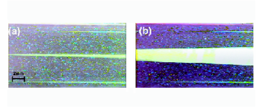
Figure 4: Example fluorescent images of the interface in an experiment from control sequence 1: (a-b) Fluid $1$ - $65\%$ saccharose solution, Fluid $2$ - $66\%$ saccharose solution, flow rate $\hat{Q}=0.145$ ml/s. The two images are separated in time by $5$ s.

The second control sequence also concerns displacement of the two fluids at neutral $pH$, i.e. without chemical reaction, but Fluid $2$ has a much larger viscosity ($\hat{\eta}_{2}\approx 20$ Pas at $\dot{\gamma}=1~{}s^{-1}$) and a significant yield stress ($\hat{\sigma}_{y}\approx 6.6$ Pa). The viscosity of Fluid $1$ is unchanged. Similar flows have been studied experimentally before in slightly larger tubes Gaba01 ; Gaba03 . As commented in Gaba01 , some care is needed in choosing the displacing flow rate, since at low flow rates the displacing fluid effectively fractures through the elastic gel, leaving a rough edge. For low flow rates we also observed a slightly granular interfacial texture and also some asymmetry of the finger. The slight asymmetry of the finger visible in Fig. 5 could be due to the non-symmetric entrance condition (the interface between fluids enters the flow channel via a $T$ shaped junction, as shown in Fig. 1) which is preserved at all later times due to the significant yield stress of Fluid $2$. Alternatively the asymmetry may relate to a transition between solid-like and fluid-like behavior. We do not attempt to explain this further.

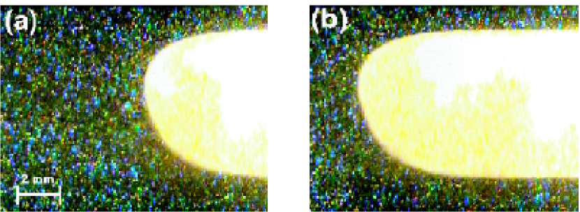
Figure 5: Example images of the interface in an experiment from control sequence $2$ ($\hat{Q}=0.08$ ml/s). Fluid $1$ has been doped with fluorescein for visualization of the fluids interface.

Sample images of an experiment in this sequence are shown in Fig. 5. The C-940 solution yields in the center of the pipe, where there is a two-dimensional flow, but the stresses are not sufficient to make it yield at the wall. Consequently a static residual wall layer is left in the tube as a finger of Fluid 1 penetrates steadily along the pipe. The shape of the nose of the finger is quite rounded and the wall layers have apparently constant thickness.

Over the duration of the experiment, there is no evidence of any interfacial instability. These results are qualitatively similar to those of Gaba01 ; Gaba03 , where C-940 solutions are displaced by glycerol solutions. The reason that there is no interfacial instability here is because the residual layers of C-940 solution are in fact fully static and unyielded. Such flows have been studied in some detail, theoretically and computationally Allo00 ; Frig01a ; Frig01c ; Frig02 , and are well understood. Even with a non-zero flow rate of C-940 solution, stable regimes may be predicted and found experimentally, see Moye04a ; Huen06 .

The two control sequences establish that without a chemical reaction and accompanying local rheology change, these displacement flows are stable. In other words, having a change in bulk rheology of the two fluids at an interface can result in instability but does not for the systems we study.

III.2 Chemically reactive unstable flows

The flow behavior was significantly different from the control experiments in the reactive case, when the C-940 solution at $pH=3$ was displaced by a saccharose solution at $pH=11$, at different flow rates. The initial interface penetrates in a sharp spike as before, but this is destabilized and the finger rapidly widens to nearly fill the pipe. A complex secondary flow develops at the interface between fluids. The flow seems to be dominated by large vortices advected by the flow, with a typical size of the order of the pipe radius. Typical images are shown in Fig. 6.

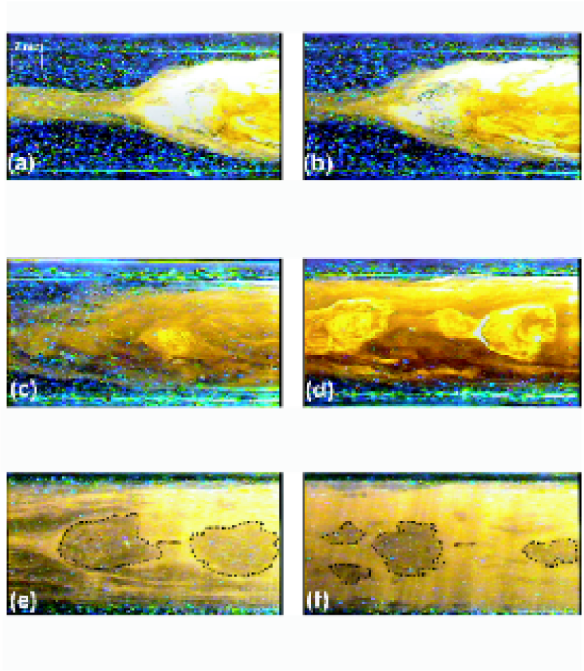
Figure 6: (a-d) Fluorescent images of the interface in a reactive displacement: Fluid $1$ - $65\%$ saccharose solution, Fluid $2$ - $0.1\%$ C-940 in $66\%$ saccharose solution. (e-f) Fluorescent flow images long after the entrance of the unstable interface in the field of view; the images are separated in time by approximately $5$ s. The dotted lines highlight gelled structures tumbling downstream.

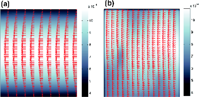
Figure 7: Instantaneous velocity fields for a chemically reactive displacement experiment, $\mathrm{Re}\approx 0.15$: (a) before entrance of the finger in the field of view (b) after the entrance of the finger in the field of view. The false color maps represent the magnitude of the velocity. In order to enhance the clarity, we only plot half of the vectors and re-scale the length of the arrows.

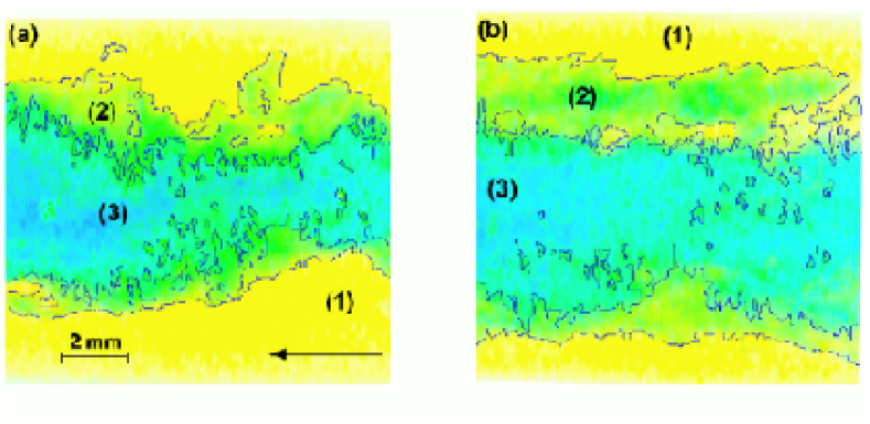
Figure 8: Iso $pH$ regions near the interface: yellow (region $1$)-$pH\approx 3$, green (region $2$)-$pH\approx 7$, blue (region $3$)-$pH\approx 11$.

As the front of the finger passes, the secondary flow instabilities persist along the sides of the finger. The secondary flow provides a feedback mechanism for the instability by bringing into contact new un-reacted fluid elements and taking away reacted highly viscous fluid. The initial pass of the finger front does not remove all the fluid $2$ from the walls. However, the secondary flows result in a fairly rapid erosion of the residual layers. After the initial instability, small parcels of Fluid 2 pulled into the Fluid 1 stream react to form gelled solid regions that are advected along with the fluid. Close observation of video images reveals that some of these parcels appear to be in rigid motion, see e.g. Fig. 6e & f.

More detailed information on the structure of velocity field is obtained from $DPIV$ images. We display in Fig. 7a & b two instantaneous velocity fields measured during a chemically reactive displacement experiment at roughly the midpoint of the fluid channel downstream. Before the entrance of the displacement front into the field of view, the flow is similar to Hagen-Poiseuille flow, see Fig. 7a. The velocity profile is parabolic and there is no secondary fluid motion in a direction orthogonal to the mean flow. Analysis of time series of velocity fields (data not shown here) has shown that the time fluctuations are only due to instrumental noise, which accounts for less than $5\%$ of the mean flow velocity. The structure of the flow field changes drastically after the passage of the displacement front through the field of view. As one can clearly see in Fig. 7b, the fluid motion follows a wavy-spiral pattern, with an apparent periodicity in the axial direction of roughly the tube diameter. The velocity field is now unstable and characterized by a rather strong radial component. Quasi-periodic entrance of slowly moving flow regions in the field of view can be associated with the passage of fully gelled solid parcels of fluid $2$ illustrated in Fig. 6e &f and discussed above.

Finally, we are able to confirm that the mixing process is locally effective and that the $pH$ varies over some intermediate range in the displacement region. To do this we image unstable flows doped with $pH$ sensitive colored dye, as shown below in Fig. 8. Since the $pH$-dependence of the fluid rheology has been characterized, in principle we could use the $DPIV$ images together with the data in Fig. 8 to construct local deviatoric stress fields. This technique however still requires some work.

III.3 Displacement efficiency

A more quantitative assessment of the displacement efficiency is obtained by processing $LIF$ images to give an indication of the evolution in time of the finger width at a fixed position along channel, roughly $50$ cm from the entrance. In each experiment a long time-series of images ($\sim 2000$) is acquired, starting long before the entrance of the displacement front into the field of view and ending long after its passage. In these experiments fluid $2$ contained Polyamide spheres and fluid $1$ a small amount of fluorescein (see section II C). The images prior to the entrance of the finger in the field of view are passed to the $DPIV$ algorithm to obtain a time series of velocity fields. The time average of these images also provides a background image that is used to compensate for non uniform illumination of each image in the sequence. The fluorescent images of the displacement front/finger are digitally processed to extract the width (measured along the radial direction) of the finger. Each image is first converted to a binary image, and the edge of the interface is detected using the $Sobel$ algorithm with a fixed brightness threshold. Spurious edge identifications, i.e. objects of the order of several pixels that are identified due to brightness inhomogeneities, are carefully removed using a morphological filter. Finally, the width of the finger is quantified from the width of the finger contour.

During reactive experiments, the instantaneous shapes of the finger are usually non-symmetric in both azimuthal and radial directions. However statistically, (considered as an ensemble average over several positions of the finger), the symmetry does not seem to break. Thus, the finger width measurement can be interpreted as a volumetric measure of the displacement efficiency, although we prefer to display time series of the width. In Fig. 9 we display the time dependence of the width of the finger for several values of flow rate. For different flow rates the time until the displacement front enters the field of view will be different. This residence time has been subtracted and the time (on the horizontal axis) is then scaled with the advection timescale, $\hat{R}/\hat{U}_{0}$. The finger width is normalized by the diameter of the pipe, $\hat{d}=2\hat{R}$.

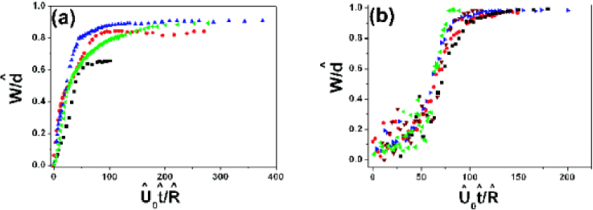
Figure 9: (a) Normalized width of the tip versus the normalized displacement distance, $\hat{U}_{0}\hat{t}/\hat{R}$, for several values of the flow rate: ($\blacksquare$) $\hat{Q}=0.063$ ml/s, ($\bullet$) $\hat{Q}=0.145$ ml/s, ($\blacktriangle$) $\hat{Q}=0.19$ ml/s, ($\blacktriangleleft$) $\hat{Q}=0.3$ ml/s. The experiments belong to Control sequence $1$ (see table 1). (b) Normalized width of the tip versus the normalized displacement distance, $\hat{U}_{0}\hat{t}/\hat{R}$, for several values of the flow rate: ($\blacktriangleleft$) $\hat{Q}=0.13$ ml/s, ($\blacksquare$) $\hat{Q}=0.18$ ml/s, ($\blacktriangledown$) $\hat{Q}=0.2$ ml/s, ($\bullet$) $\hat{Q}=0.31$ ml/s, ($\blacktriangleright$) $\hat{Q}=0.47$ ml/s. The experiments belong to the Reactive sequence (see Table 1).

Fig. 9a shows the normalized width of the finger, $W/\hat{d}$, for the experiments in control sequence $1$, where two Newtonian fluids are displaced. For each flow rate, $W/\hat{d}$ saturates at values smaller than unity, indicating that in all cases fluid $2$ was only partially displaced. Qualitatively similar results are given in Peti96 . Fig. 9b shows analogous results for the reactive displacements at different flow rates. The interfacial instability clearly results in an efficient mass transport in the cross flow direction. For each flow rate, $W/\hat{d}$ saturates at values very close to unity. Observe that the initial points on the time series are noisy, followed by a rapid increase to near saturation, then slow approach to unity as the wall layers are consumed by the secondary flows/instability. The initial noisy part of the curves corresponds to destabilization of the initial interfacial spike.

In comparing these two figures, recall that the time axis has been shifted to correspond to the initial appearance of fluid $1$. In the case of the unstable displacements, this is harder to determine precisely due to the destabilized wispy spike. Once the bulk of the displacing finger arrives, the rapid increase to near the saturation values is similar in both cases. The wider spread of the curves in Fig. 9b is due to the early arrival of the initial spike and slower erosion of the final wall layer. In terms of a volumetric measure of efficiency, the reactive displacement leaves $\lesssim 5\%$ of the displaced fluid volume, and this appears to be insensitive to the flow rate. The stable Newtonian displacements leave between $20\%$ and $60\%$ of the displaced fluid in the pipe, with strong dependence on the flow rate.

The key observations of Fig. 9b is that all the efficiency curves (time shifted for arrival) have similar shape and that the time scales with $\hat{R}/\hat{U}_{0}$. In terms of an averaged volumetric concentration of displaced fluid, say $\bar{C}(\hat{x},\hat{t})=(W/\hat{d})^{2}$, this suggests a functional form:

$$\bar{C}(\hat{x},\hat{t})=\bar{C}(\hat{x}-\hat{U}_{0}\hat{t},\hat{t}\hat{U}_{0}/\hat{R}),$$

and the sigmoid shape is reminiscent of axial dispersion in a moving frame of reference. If this dispersion is governed by an axial diffusivity $\hat{D}_{a}$, the timescale for the spreading is $\hat{t}\sim\hat{R}^{2}/\hat{D}_{a}$. Thus, the collapse of our data with respect to the time variable $\hat{R}/\hat{U}_{0}$, suggests the scaling law

$$\hat{D}_{a}\sim\hat{R}\hat{U}_{0},$$

which infers a similar scaling law for a transverse diffusivity of mixing, $\hat{D}_{r}$, see §I.1.

Even if redrawn volumetrically, the curves in Fig. 9b are not symmetric about the mid-concentration. Additionally, close inspection reveals small differences between the curves for different flow rates. These suggest that, although axial dispersion may provide a reasonable leading order model, the dispersion coefficient will vary nonlinearly with respect to $\bar{C}$ and have other weak dependencies. This is in fact physically obvious: the mechanism governing the initial instability of the wispy spike ($\bar{C}\sim 0$) is clearly quite different to that governing erosion/break up of the residual wall layer of C-940 ($\bar{C}\sim 1$).

IV Hydrodynamic instabilities driven by viscosity gradients

We would like to understand better the origin of the instabilities that develop into secondary flows such as those in Fig. 6. Development of a complete stability analysis of the reaction-diffusion system coupled to the hydrodynamics is a formidable task, and perhaps unnecessary. One obstacle is that the reaction kinetics are not fully quantified. Another obstacle is to fully understand the coupling between the reaction and the hydrodynamics. This analysis is however underway and we hope to report the results later. For now, we offer some insights via analysis of a simpler toy problem.

First, we note that the chemical reaction occurs on a time scale $\hat{t}_{ch}$ which is much shorter than the hydrodynamic time scales of the problem. This is supported by the estimation below.

Following ref. Atkins , the characteristic time scale at which the chemical reaction occurs is roughly $\hat{t}_{ch}\approx 10^{-9}$s. In our experiments, the characteristic hydrodynamic times are the diffusion time, $\hat{t}_{D}=\hat{R}^{2}/\hat{D}$, the advection time, $\hat{t}_{a}=\hat{R}/\hat{U}_{0}$, and the viscous time, $\hat{t}_{v}=\hat{\rho}\hat{R}^{2}/\hat{\eta}_{0}$. If one considers $\hat{D}\approx 4.2\cdot 10^{-12}~{}\text{m}^{2}/\text{s}$ (which is roughly the diffusion coefficient of fluorescein in our solutions) and $\hat{U}_{0}\approx 5~{}\text{mm/s}$ (which corresponds to half of our experimental range), one can estimate $\hat{t}_{D}\approx 7.2\cdot 10^{6}$ s, $\hat{t}_{a}\approx 1.1$ s and $\hat{t}_{v}\approx 0.3$ s. The numerical estimates above show a clear separation of time scales in our problem: $\hat{t}_{ch}\ll\hat{t}_{v}<\hat{t}_{a}\ll\hat{t}_{D}$. In view of this, it is reasonable to assume that the fast reaction instantaneously establishes an initial concentration profile when two fluids come into contact. This ”reaction front” is a diffuse layer of reacted fluid separating the two bulk fluids, within which the $pH$ is approximately neutral and the viscosity is consequently elevated. In the following we will investigate the hydrodynamic stability of such a viscosity profile.

This process is on the slow scale of $t_{a}$. Note that the reaction is not auto-catalytic. Unless there is convective motion that brings fresh un-reacted fluids into contact, the reaction front broadens diffusively. No self-sustaining traveling chemical waves arise. In addition, unlike the many ”chemical reaction plus buoyancy” studied referenced in §I, our fluids have matching densities that are unchanged by the reaction. Consequently, there is no momentum source resulting from the reaction. Therefore, the direct effect of the continual reaction is to create a source term in the advection-diffusion equation for the concentration. Indirectly this modifies the viscosity profile. For simplicity, however, we will ignore the effects of continual reaction, and focus on the fate of the initial, chemically created, concentration and viscosity profiles.

Figure 10: Example basic viscosity and velocity profiles for $c_{0}=0.5$, $\Delta c_{0}=0.1$ and $a=100$: (a) Normalized base viscosity profile. (b) Normalized base velocity profile.

Furthermore we ignore the pipe geometry , and consider instead a symmetric plane Poiseuille flow in a channel of width $2\hat{R}$ along which fluid is pumped at mean speed $\hat{U}_{0}$. The fluid is assumed to have a concentration dependent viscosity $\hat{\eta}(c)$ that consists of a base viscosity $\hat{\eta}_{0}$ that is augmented (by a factor $a$) over some finite range of concentrations, $\Delta c_{0}$, close to a fixed concentration value $c=c_{0}$. For example, one such function would be:

$$\hat{\eta}(c)=\hat{\eta}_{0}\left[1+a\cos^{4}\left(\frac{\pi(c-c_{0})}{2\Delta c_{0}}\right)\right],$$

which is depicted in Fig. 10a. Ignoring the reaction, the concentration satisfies an advection-diffusion equation and the fluid flow satisfies the Navier-Stokes equations. There exists a steady base flow in which the concentration varies linearly across the channel. The increased viscosity tends to flatten the base Poiseuille velocity profile within the diffuse layer, see e.g. Fig. 10b.

We consider the linear stability of this base flow, using classical methods. The stability problem is governed by the Reynolds number $\mathrm{Re}=(\hat{\rho}\hat{R}\hat{U}_{0})/\hat{\eta}_{0}\lesssim 1$, the Schmidt number, $\mathrm{Sc}=\hat{\eta}_{0}/(\hat{\rho}\hat{D})\in[10^{4},10^{6}]$, the initial concentration profile $C_{0}$, the layer thickness and position, $\Delta c_{0}$ & $c_{0}$, and the amplitude $a$ of the viscosity jump. Introducing the non-dimensional variables

$$x=\frac{\hat{x}}{\hat{R}},\quad y=\frac{\hat{y}}{\hat{R}},\quad t=\frac{\hat{t}}{\hat{t}_{v}},\quad U=\frac{\hat{U}}{\hat{U}_{0}},\quad\eta=\frac{\hat{\eta}}{\hat{\eta}_{0}}$$

the growth or decay of a linear mode $(f(y),c(y))e^{i\alpha x+\sigma t}$ is governed by the following eigenvalue problem:

$$\sigma\left(D^{2}-\alpha^{2}\right)f = \frac{1}{\mathrm{Re}}L_{1}f+L_{2}f+L_{3}c$$ (4)

$$\sigma c = i\alpha\mathrm{Re}\;\Bigl{(}(DC_{0})f-Uc\Bigr{)}+\frac{1}{\mathrm{Sc}}\left(D^{2}-\alpha^{2}\right)c$$ (5)

where $D=d/dy$, $\eta=\eta(C_{0})$, $C_{0}=1-y$, and

$$L_{1} := -i\alpha\Bigl{(}U(D^{2}-\alpha^{2})-(D^{2}U)\Bigr{)}$$

$$L_{2} := (D^{2}\eta)\left(D^{2}+\alpha^{2}\right)+2(D\eta)D\left(D^{2}-\alpha^{2}\right)+\eta\left(D^{2}-\alpha^{2}\right)^{2}$$

$$L_{3} := D^{2}\left(\frac{\partial\eta}{\partial C_{0}}DU\right)I+2D\left(\frac{\partial\eta}{\partial C_{0}}DU\right)D+\left(\frac{\partial\eta}{\partial C_{0}}DU\right)(D^{2}+\alpha^{2})$$

We discretize the equations using Chebyschev polynomials and determine the maximal growth rates $\sigma_{R}$ as a function of wave number $\alpha$ (and the other dimensionless parameters), in the standard way, see e.g. Schmid . Examples of the results are shown below.

IV.1 Results

Typically in our experiments we have $\mathrm{Re}\lesssim 1$, so that we are far below the range for inertia-driven shear instabilities. If $a=0$, the viscosity is constant so that equation (4) decouples and reduces to the classical Orr-Sommerfeld equation, which is stable at low $\mathrm{Re}$. Equation (5) then gives only stable modes with $\sigma_{R}<0$ decreasing quadratically with $\alpha$. As the amplitude $a$ increases, unstable modes are found over an increasing range of $\alpha$, including the long wave limit $\alpha=0$, with diffusion stabilizing the short wavelengths. Figure 11 shows typical examples of the growth rate $\sigma_{R}$ vs $\alpha$, for a range of different $a$, at two different values of $\mathrm{Sc}$.

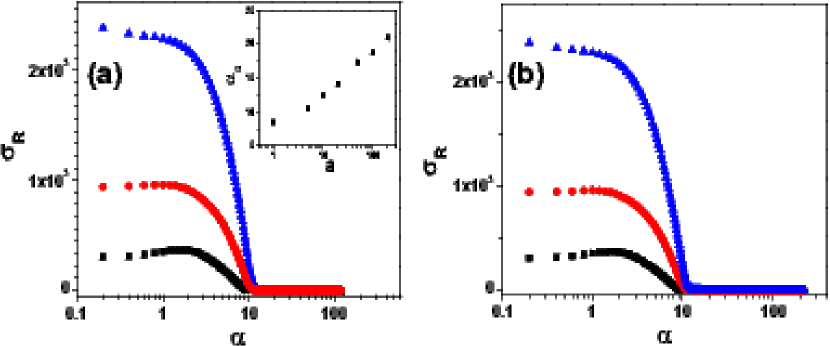
Figure 11: Example results: $\sigma_{R}$ vs $\alpha$ for the base flow of Fig. 10 with the viscosity amplitudes ($\blacktriangle$) $a=100$ ($\blacksquare$) $a=5$ and ($\bullet$) $a=20$: (a) $\mathrm{Sc}=10^{4}$. In the inset we display the dependence of the critical wave number, $\alpha_{c}$, on the amplitude $a$; (b) $\mathrm{Sc}=10^{6}$.

The long wave limit $\alpha\to 0$ tends to give the largest growth rates, but these modes will not be excited in a developing finger-like displacement. Unstable wave numbers are found up to a critical wave number $\alpha_{c}$, which varies with $a$ and $\Delta c_{0}$, increasing mildly with $a$. A possible physical interpretation of the ($x$-independent) long wavelength instability is simply that a different base flow may exist and be somehow more stable. In order to compare with the experimental results, note that the wave numbers are scaled with $\hat{R}^{-1}$ and the growth rates with the inverse viscous timescale, $\hat{t}_{v}$, (which is $\approx 0.3$ s for our experiments). Thus, we can see from Fig. 11 that wavelengths $\sim\hat{R}$ are certainly excited at viscosity amplifications $a=100$. The growth rates are very rapid and we would therefore not expect to see linear modal effects.

A complete exploration of the parameter space of this problem does not seem worthwhile and is not easy numerically. Although we typically have large $\mathrm{Sc}$, the limit $\mathrm{Sc}\to\infty$ results in loss of the diffusive terms in the concentration equation and it is these that stabilize the short wavelengths. The other limits of large $a$ and small $\Delta c_{0}$ will obviously eventually cause problems for the Chebyschev expansion, and would be better investigated analytically, as would the large and small wave number limits.

V Discussion and Conclusions

In this study we have presented experimental evidence of an inertial free shear flow instability caused by changes in the local fluid rheology. We have focused on low $\mathrm{Re}$ number displacement flows in an horizontal pipe. An acid-base type chemical reaction occurs near the interface between fluids and results in molecular reorganization of the Carbopol-940 (C-940) polymer. The main result of this molecular reorganization is the formation of a stiff gel, characterized by a large viscosity and a significant yield stress.

In order to test the effect of these rheological changes on the hydrodynamic stability of the flow, we have carried out two control experimental sequences, see Table 1 series $1$ and $2$. In neither of the control experiments was a flow instability observed. If both fluids were Newtonian (first control sequence), the displacement flow was dominated by a long finger of fluid $1$ penetrating into fluid $2$, Fig. 4. The flow was stable and the second fluid was never completely removed from the channel walls, Fig. 9a. If the displaced fluid was a yield stress fluid, the flow remained stable at all times, (second control sequence), see Fig. 5.

The behavior was significantly different in the reactive case. The interface between the fluids becomes unstable and mixes across the entire channel. The flow fields are unsteady and characterized by a strong secondary motion in a direction orthogonal to the mean flow direction, Fig. 7b. The relevance of our experimental findings is threefold.

1. First, the coupling between chemical reaction and a strong non-monotonic local change in the fluid rheology is novel. For simple fluids, viscosity variations can be caused by temperature or concentration gradients, but these tend to be gradual and monotone. Use of complex fluids allows one to localize the change in viscosity and produce non-monotone effects.
   The instability mechanism we have described in this paper is not restricted to interfacial flows, where acid-base type chemical reactions take place at the interface between two fluids via transport of unbalanced charges across the interface. Similar chemical reactions, which result in significant changes in the fluid rheology, may be triggered in a non invasive way, e.g. by exposing fluid parcels to either electromagnetic radiation or heat waves which will locally initiate a polymerization reaction. For example, there exist numerous polymeric materials (epoxies) widely used in photo lithography, whose viscosity increases dramatically (up to solidification, depending on the chemical nature of the polymer and the exposure conditions) upon exposure to monochromatic electromagnetic radiation. Also, liquid silicone elastomers may display a similar behavior (they turn from viscous liquid state to solid elastic) when locally heated. This observation, together with an instability mechanism similar to the one illustrated in this paper, may open new possibilities of externally controlling the hydrodynamic stability of inertia free shear flows.

2. Secondly, we have demonstrated a significant increase in the displacement efficiency for reactive displacements. This has an impact on process applications such as these described in §I.1, and this was the initial motivation for our study.

3. Thirdly, we have demonstrated a new mechanism for low $\mathrm{Re}$ mixing that does not require large inertial energies. This in itself opens up many interesting avenues for practical applications, e.g. mixing in micro-fluidic flows. Indeed, efficient mixing in the absence of inertia requires an additional mechanism than molecular diffusion (which is the least efficient). Several micro mixing techniques have been proposed during the past half decade, all based on different mechanisms of generating secondary flows (steady or random in time). One of these techniques is based on the recently discovered elastic turbulence  etnature , which is a random (in time) and complex dynamic flow state in dilute solutions of linear flexible polymers. As shown in mixingnature ; mixingPRE , elastic turbulence can be successfully employed in efficiently mixing viscous fluids in the absence of inertia. Although the flow configuration we used in this study is not a typical mixing configuration, based on the data presented in Figs. 6, and 8, one can suggest that the instability discussed in this paper could be alternatively used as a low $\mathrm{Re}$ mixing method.

Our hydrodynamic stability study is minimalist and we have presented only brief results. However, the simple toy model shows that long wavelength instabilities do result from non-monotonic viscosity variations of the magnitude that we have and in the correct range of $\mathrm{Re}$ and $\mathrm{Sc}$. A more detailed study of these reactive displacements is underway.

- (1) H. Bénard, “Les tourbillons cellulaires dans une nappe liquide,” Rev. Gén. Sci. pures et appl. 11, 1261 (1900).
- (2) L. Landau and E. Lifschitz, Fluid Mechanics (Pergamon Press, Oxford, 1987).
- (3) P. Ern, F. Charru, and P. Luchini, “Stability analysis of a shear flow with strongly stratified viscosity,” J. Fluid Mech. 496, 295 (2003).
- (4) C. Tan and G. Homsy, “Stability of miscible displacements in porous media: Rectilinear flow,” Phys. Fluids 29, 3549 (1986).
- (5) F. Hickernell and Y. C. Yortsos, “Linear stability of miscible displacement processes in porous media in the absence of dispersion,” Stud. Appl. Math. 74, 93 (1986).
- (6) S. Chang and J. Slattery, “A linear stability analysis for miscible displacements,” Trans. Porous Media 1, 179 (1986).
- (7) Y. C. Yortsos, “Stability of displacement processes in porous media in radial flow geometries.” Phys. Fluids 30, 2928 (1987).
- (8) C. Tan and G. Homsy, “Simulation of nonlinear viscous fingering viscous fingering in miscible displacement,” Phys. Fluids 31, 1330 (1988).
- (9) Y. C. Yortsos and M. Zeybek, “Dispersion driven instability in miscible displacement in porous media.” Phys. Fluids 31, 3511 (1988).
- (10) P. Petitjeans and T. Maxworthy, “Miscible displacements in capillary tubes. Part 1. Experiments,” J. Fluid Mech. 326, 37 (1996).
- (11) C.-Y. Chen and E. Meiburg, “Miscible displacements in capillary tubes. Part 2. Numerical simulations,” J. Fluid Mech. 326, 81 (1996).
- (12) N. Rakotomalala, D. Salin, and P. Watzky, “Miscible displacement between two parallel plates: BGK lattice gas simulations.” J. Fluid Mech. 338, 277 (1997).
- (13) Z. Yang and Y. C. Yortsos, “Asymptotic solutions of miscible displacements in geometries of large aspect ratio,” Phys. Fluids 9, 286 (1997).
- (14) E. Lajeunesse, J. Martin, N. Rakotomalala, D. Salin, and Y. Yortsos, “Miscible displacement in a Hele Shaw cell at high rates,” J. Fluid Mech. 398, 299 (1999).
- (15) C.-S. Yih, “Instability due to viscosity stratification,” J. Fluid Mech. 27, 337 (1967).
- (16) C. Hickox, “Instability due to viscosity and density stratification in axisymmetric pipe flow,” Phys. Fluids 14, 251 (1971).
- (17) D. Joseph and Y. Renardy, Fundamentals of Two-Fluid Dynamics. (Interdisciplinary Applied Mathematics, Springer, 1993).
- (18) E. Hinch, “A note on the mechanism of the instability at the interface between two shearing fluids,” J. Fluid Mech. 114, 463 (1984).
- (19) F. Charru and E. Hinch, “”phase diagram” of interfacial instabilities in a two-layer Couette flow and mechanism of the long wave instability,” J. Fluid Mech. 414, 195 (2000).
- (20) E. Chikhliwala, A. Huang, and Y. C. Yortsos, “Numerical study of the linear stability of immiscible displacement in porous media,” Trans. Porous Media 3, 257 (1988).
- (21) O. Manickam and G. Homsy, “Stability of miscible displacements in porous media with nonmonotonic viscosity profiles,” Phys. Fluids 5, 1356 (1993).
- (22) R. B. Bird, C. F. Curtiss, R. C. Armstrong, and O. Hassager, Dynamics of Polymeric Liquids, vol. 2 (John Wiley, NY, 1987).
- (23) J. Tyson and J. Keener, “Singular perturbation theory of travelling waves in excitable media (a review),” Physica D 32, 327 (1988).
- (24) J. A. Pojman and I. R. Epstein, “Convective effects on chemical waves. 1.: Mechanisms and stability criteria,” J. Phys. Chem. 94, 4966 (1990).
- (25) B. Edwards, J. Wilder, and S. K., “Onset of convective for autocatalytic reaction fronts: Laterally unbounded systems,” Phys. Rev. A 43, 749 (1991).
- (26) D. Vasquez, B. Edwards, and J. Wilder, “Onset of convective for autocatalytic reaction fronts: Laterally bounded systems,” Phys. Rev. A 43, 6694 (1991).
- (27) D. Vasquez, J. Littley, J. Wilder, and B. Edwards, “Convection in chemical waves,” Phys. Rev. E 51, 280 (1994).
- (28) B. Edwards, “Poiseuille advection of chemical reaction fronts,” Phys. Rev. Lett. 89 (2002).
- (29) D. Vasquez and A. De Wit, “Dispersion relations for the convective instability of an acidity front in Hele-Shaw cells,” J. Chem. Phys. 121 (2001).
- (30) J. D’Hernoncourt, A. Zebib, and A. De Wit, “Reaction driven convection around a stably stratified chemical front,” Phys. Rev. Lett. 96 (2006).
- (31) D. Lima, A. D’Onfrio, and A. De Wit, “Nonlinear fingering dynamics of reaction-diffusion fronts: Self-similar scaling and influence of differential diffusion,” J. Chem. Phys. 124 (2006).
- (32) A. De Wit and G. Homsy, “Viscous fingering in periodically heterogeneous porous media. I. Formulation and linear instability,” J. Chem. Phys. 107, 9609 (1997).
- (33) A. De Wit and G. Homsy, “Viscous fingering in periodically heterogeneous porous media. II. Numerical simulations,” J. Chem. Phys. 107, 9619 (1997).
- (34) A. De Wit and G. Homsy, “Nonlinear interactions of chemical reactions and viscous fingering in porous media,” Phys. Fluids 11, 949 (1999).
- (35) A. De Wit and G. Homsy, “Viscous fingering in reaction-diffusion systems,” J. Chem. Phys. 110, 8663 (1999).
- (36) A. Bourgoyne, K. Millheim, and M. Chenever, Applied Drilling Engineering Textbook, vol. 2 of ISBN: 1-55563-001-4 (Society of Petroleum Engineers).
- (37) Pore Pressure and Fracture Gradients Reprint No.49, ISBN: 1-55563-081-2 (Society of Petroleum Engineers, 1999).
- (38) Horizontal Wells Reprint No.47, ISBN: 1-55563-076-6 (Society of Petroleum Engineers, 1998).
- (39) E. B. Nelson, Well Cementing (Schlumberger Educational Services., 1990).
- (40) F. Scarano and M. L. Rhiethmuller, “Advances in iterative multigrid PIV image processing,” Exp. Fluids 29 (2001).
- (41) F. K. Oppong, L. Rubatat, B. Frisken, A. Bailey, and J. de Bruyn, “Microrheology and structure of a yield-stress polymer gel.” Phys. Rev. E 73, 041405 (2006).
- (42) G. C., “Etude de la stabilité de films liquides sur les parois d’une conduite verticale lors de l’ecoulement de fluides miscibles non-newtoniens.” (2001), these de l’Universite Pierre et Marie Curie (PhD thesis), Orsay, France.
- (43) C. Gabard and J.-P. Hulin, “Miscible displacements of non-Newtonian fluids in a vertical tube,” Eur. Phys. J. E 11, 231 (2003).
- (44) M. Allouche, I. Frigaard, and G. Sona, “Static wall layers in the displacement of two visco-plastic fluids in a plane channel,” J. Fluid Mech. 424, 243 (2000).
- (45) I. Frigaard, S. O., and S. G., “Uniqueness and non-uniqueness in the steady displacement of two viscoplastic fluids,” ZAMM 81, 99 (2001).
- (46) I. Frigaard, “Super-stable parallel flows of multiple visco-plastic fluids,” J. Non-Newtonian Fluid Mech. 100, 49 (2001).
- (47) I. Frigaard, L. S., and S. O., “Variational methods and maximal residual wall layers,” J. Fluid Mech. 483, 37 (2003).
- (48) M. Moyers-Gonzalez, I. A. Frigaard, and C. Nouar, “Nonlinear stability of a visco-plastically lubricated viscous shear flow,” J. Fluid Mech. 506, 117 (2004).
- (49) C. Huen, I. Frigaard, and D. Martinez, “Experimental studies of multi-layer flows using a viscoplastic lubricant,” J. Non-Newtonian Fluid Mech. in press (2006).
- (50) P. W. Atkins and J. W. Locke, Physical Chemistry (Oxford University Press, 2002).
- (51) P. J. Schmid and D. S. Henningson, Stability and Transition in Shear Flows, vol. 142 of Applied Mathematical Sciences (Springer, 2001).
- (52) A. Groismann and V. Steinberg, “Elastic turbulence in a polymer solution flow,” Nature 405, 53 (2000).
- (53) A. Groisman and V. Steinberg, “Efficient mixing at low Reynolds numbers using polymer additives,” Nature 410, 905 (2001).
- (54) T. Burghelea, E. Segre, I. Bar-Joseph, A. Groisman, and V. Steinberg, “Chaotic flow and efficient mixing in a microchannel with a polymer solution.” Phys. Rev. E 69, 066305 (2004).