Modelling train delays with $q$-exponential functions

Abstract

We demonstrate that the distribution of train delays on the British railway network is accurately described by $q$-exponential functions. We explain this by constructing an underlying superstatistical model.

1 Introduction

Complex systems in physics, engineering, biology, economics, and finance, are often characterized by the occurence of fat-tailed probability distributions. In many cases there is an asymptotic decay with a power-law. For these types of systems more general versions of statistical mechanics have been developed, in which power laws are effectively derived from maximization principles of more general entropy functions, subject to suitable constraints [1, 2, 3, 4]. Typical distributions that occur in this context are of the $q$-exponential form. The $q$-exponential is defined as $e_{q}(x):=(1+(q-1)x)^{1/(q-1)}$, where $q$ is a real parameter, the entropic index. It has become common to call the corresponding statistics ‘$q$-statistics’.

A possible dynamical reason for $q$-statistics is a so-called superstatistics [5]. For superstatistical complex systems one has a superposition of ordinary local equilibrium statistical mechanics in local spatial cells, but there is a suitable intensive parameter $\beta$ of the complex system that fluctuates on a relatively large spatio-temporal scale. This intensive parameter may be the inverse temperature, or the amplitude of noise in the system, or the energy dissipation in turbulent flows, or an environmental parameter, or simply a local variance parameter extracted from a suitable time series generated by the complex system [6]. The superstatistics approach has been the subject of various recent papers [7, 8, 9, 10, 11, 12] and it has been applied to a variety of complex driven systems, such as Lagrangian[13, 14] and Eulerian turbulence[15, 6], defect turbulence[16], cosmic ray statistics[17], solar flares [18], environmental turbulence [19], hydroclimatic fluctuations [20], random networks [21], random matrix theory [22] and econophysics [23].

If the parameter $\beta$ is distributed according to a particular probability distribution, the $\chi^{2}$-distribution, then the corresponding superstatistics, obtained by integrating over all $\beta$, is given by $q$-statistics [1, 2, 3, 4], which means that there are $q$-exponentials and asymptotic power laws. For other distributions of the intensive parameter $\beta$, one ends up with more general asymptotic decays [8].

In this paper we intend to analyse yet another complex system where $q$-statistics seem to play an important role, and where a superstatistical model makes sense. We have analysed in detail the probability distributions of delays occuring on the British rail network. The advent of real-time train information on the internet for the British network (http://www.nationalrail.co.uk/ ldb/livedepartures.asp) has made it possible to gather a large amount of data and therefore to study the distribution of delays. Information on such delays is very valuable to the traveller. Published information is limited to a single point of the distribution - for example, the fraction of trains that arrive with 5 minutes of their scheduled time. Travellers thus have no information about whether the distribution has a long tail, or even about the mean delay. We find that the delays are well modelled by a $q$-exponential function, allowing a characterization of the distribution by two parameters, $q$ and $b$. We will relate our observations to a superstatistical model of train delays.

This paper is organized as follows: first, we describe our data and the methods used for the analysis. We then present our fitting results. In particular, we will demonstrate that $q$-exponentials provide a good fit of the train delay distributions, and we will show which parameters $(q,b)$ are relevant for the various British rail network lines. In the final section, we will discuss a superstatistical model for train delays.

2 The data

We collected data on departure times for 23 major stations for the period September 2005 to October 2006, by software which downloads the real-time information webpage every minute for each station. As each train actually departs, the most recent delay value is saved to a database. The database now contains over two million train departures; for a busy station such as Manchester Piccadilly over 200,000 departures are recorded.

3 The model and parameter estimation

Preliminary investigation led us to believe that the model

$$e_{q,b,c}(t)=c(1+b(q-1)t)^{1/(1-q)}$$ (1)

would fit well; here $t$ is the delay, $0\!<q\!<2$ and $b\!>\!0$ are shape parameters, and $c$ is a normalization parameter. We have $e_{q,b,c}(t)=c(1-bt)+O(t^{2})$ as $t\rightarrow 0$ and $\log(e_{q,b,c}(t))/\log(t)\rightarrow 1/(1-q)$ as $t\rightarrow\infty$. These limiting forms allow an initial estimate of the parameters; an accurate estimate is then obtained by nonlinear least-squares. We also have

$$\lim_{q\rightarrow 1}e_{q,b,c}(t)=c\exp(-bt),$$ (2)

so that $q$ measures the deviation from an exponential distribution. An estimated $q$ larger than unity indicates a long-tailed distribution.

We did not include the zero-delay value in the fitted models. Typically 80% of trains record $t=0$, indicating a delay of one minute or less (the resolution of the data). Thus, our model represents the conditional probability distribution of the delay, given that the train is delayed one minute or more.

In order to provide meaningful parameter confidence intervals, we weighted the data as follows. Since our data is in the form of a histogram, the distribution of the height $c_{i}$ of the bar representing the count of trains with delay $i$ will be binomial. In fact, it is of course very close to Gaussian whenever $c_{i}$ is large enough, which is the case nearly always. The normalized height $f_{i}=c_{i}/n$ (where $n$ is the total number of trains) will therefore have standard deviation $\sigma_{i}=(nf_{i}(1-f_{i}))^{1/2}/n\approx c_{i}^{1/2}/n$. We used these values as weights in the nonlinear least squares procedure, and hence computed parameter confidence intervals by standard methods, namely from the estimated parameter covariance matrix. We find that typically $q$ and $b$ have a correlation coefficient of about $-0.5$; thus, the very small confidence intervals quoted in the figure captions for $b$ are not particularly useful; $b$ typically acquires a larger uncertainty via its correlation with $q$.

4 Results

We first fitted the model to all data, obtaining the fit shown in Figure 1. This corresponds to a ‘universality’ assumption - if all routes had the same distribution of delays, the parameter values $q=1.355,b=0.524$ would be the relevant ones. We may thus compare the parameters for specific routes with these. Typical fits for three such routes are shown in Fig. 2, Fig. 3, and Fig. 4.

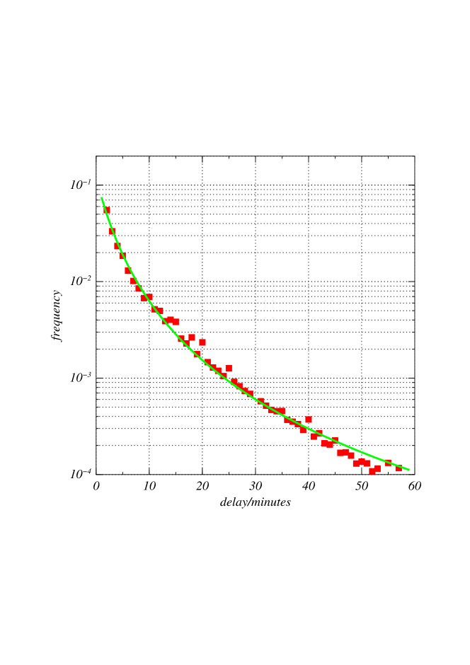
Figure 1: All train data and best-fit $q$-exponential: $q=1.355\pm 8.8\times 10^{-5}$, $b=0.524\pm 2.5\times 10^{-8}$.

Delays typically build up over a train’s journey, and are very unlikely at the initial departure station. Thus, we choose to study delays at intermediate stations. At such stations, a delayed departure almost certainly means the arrival was delayed.

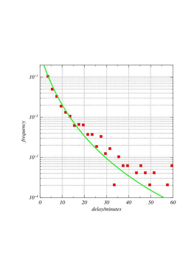
Figure 2: Bath Spa to London Paddington (showing typical fluctuations in the tail when data is sparse): $q=1.215\pm 0.015$, $b=0.405\pm 2.8\times 10^{-6}$.

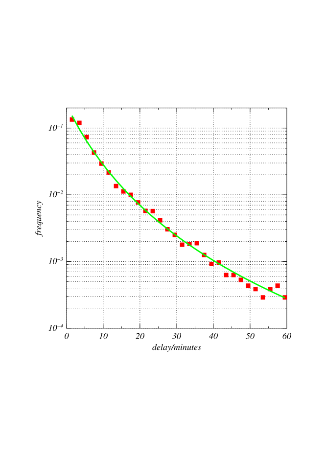
Figure 3: Swindon to London Paddington: $q=1.230\pm 0.0086$, $b=0.266\pm 3.1\times 10^{-6}$.

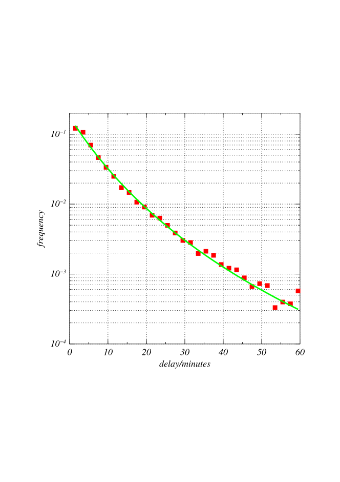
Figure 4: Reading to London Paddington: $q=1.183\pm 0.0063$, $b=0.202\pm 2.7\times 10^{-6}$.

5 Superstatistical model

We start with a very simple model for the local departure statistics of trains. The waiting time distribution until departure takes place is simply given by that of a Poisson process [24]

$$P(t|\beta)=\beta e^{-\beta t}.$$ (3)

Here $t$ is the time delay from the scheduled departure time, and $\beta$ is a positive parameter. The symbol $P(t|\beta)$ denotes the conditional probability density to observe the delay $t$ provided the parameter $\beta$ has a certain given value. Clearly, the above probability density is normalized. Large values of $\beta$ mean that most trains depart very well in time, whereas small $\beta$ describe a situation where long delays are rather frequent.

The above simple exponential model becomes superstatistical by making the parameter $\beta$ a fluctuating random variable as well. These fluctuations describe large-scale temporal variations of the British rail network environment. For example, during the start of the holiday season, when there is many passengers, we expect that $\beta$ is smaller than usual for a while, resulting in frequent delays. Similarly, if there is a problem with the track or if bad weather conditions exist, we also expect smaller values of $\beta$ on average. The value of $\beta$ is also be influenced by extreme events such as derailments, industrial action, terror alerts, etc.

The observed long-term distribution of train delays is then a mixture of exponential distributions where the parameter $\beta$ fluctuates. If $\beta$ is distributed with probability density $f(\beta)$, and fluctuates on a large time scale, then one obtains the marginal distributions of train delays as

$$p(t)=\int_{0}^{\infty}f(\beta)p(t|\beta)d\beta=\int_{0}^{\infty}f(\beta)\beta e^{-\beta t}.$$ (4)

It is this marginal distribution that is actually recorded in our data files.

Let us now construct a simple model for the distribution $f(\beta)$. There may be $n$ different Gaussian random variables $X_{i},i=1,\ldots,n$, that influence the dynamics of the positive random variable $\beta$ in an additive way [25]. We may thus assume as a very simple model that

$$\beta=\sum_{i=1}^{n}X_{i}^{2},$$ (5)

where $\langle X_{i}\rangle=0$ and $\langle X_{i}^{2}\rangle\not=0$. In this case the probability density of $\beta$ is given by a $\chi^{2}$-distribution with $n$ degrees of freedom:

$$f(\beta)=\frac{1}{\Gamma\left(\frac{n}{2}\right)}\left(\frac{n}{2\beta_{0}}\right)^{\frac{n}{2}}\beta^{\frac{n}{2}-1}\exp\left(-\frac{n\beta}{2\beta_{0}}\right).$$ (6)

The average of $\beta$ is given by

$$\langle\beta\rangle=n\langle X_{i}^{2}\rangle=\int_{0}^{\infty}\beta f(\beta)d\beta=\beta_{0}$$ (7)

and the variance by

$$\langle\beta^{2}\rangle-\beta_{0}^{2}=\frac{2}{n}\beta_{0}^{2}.$$ (8)

The integral (4) is easily evaluated and one obtains

$$p(t)\sim{\left(1+b(q-1)t\right)^{\frac{1}{1-q}}}$$ (9)

where $q=1+{2}/(n+2)$ and $b={2}\beta_{0}/({2-q})$. Our model generates $q$-exponential distributions of train delays by a simple mechanism, namely a $\chi^{2}$-distributed parameter $\beta$ of the local Poisson process.

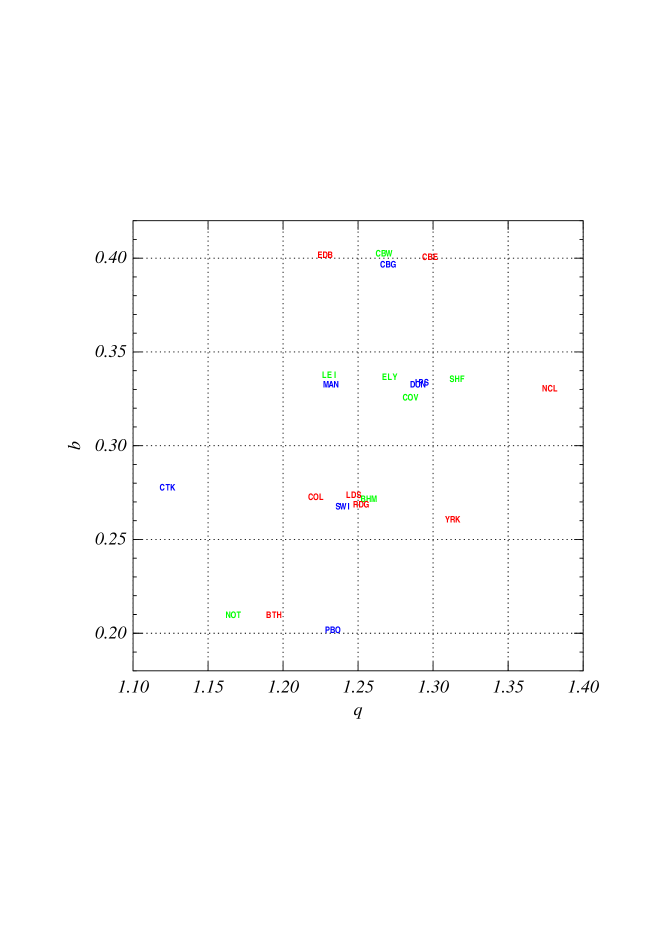
Figure 5: The estimated parameters $q$ and $b$ for 23 stations.

station	$q$	$b$	code
Bath Spa	1.195	0.209	BTH
Birmingham	1.257	0.271	BHM
Cambridge	1.270	0.396	CBG
Canterbury East	1.298	0.400	CBE
Canterbury West	1.267	0.402	CBW
City Thameslink	1.124	0.277	CTK
Colchester	1.222	0.272	COL
Coventry	1.291	0.330	COV
Doncaster	1.289	0.332	DON
Edinburgh	1.228	0.401	EDB
Ely	1.316	0.393	ELY
Ipswich	1.291	0.333	IPS
Leeds	1.247	0.273	LDS
Leicester	1.231	0.337	LEI
Manchester Piccadilly	1.231	0.332	MAN
Newcastle	1.378	0.330	NCL
Nottingham	1.166	0.209	NOT
Oxford	1.046	0.141	OXF
Peterborough	1.232	0.201	PBO
Reading	1.251	0.268	RDG
Sheffield	1.316	0.335	SHF
Swindon	1.226	0.253	SWI
York	1.311	0.259	YRK

Table 1: The estimated parameters $q$ and $b$ for 23 stations.

Typical $q$-values obtained from our fits are in the region $q=1.15\dots 1.35$ (see Fig. 5 and Table 1). This means

$$n=\frac{2}{q-1}-2$$ (10)

is in the region $4\ldots 11$. This means the number of degrees of freedom influencing the value of $\beta$ is just of the order we expected it to be: A few large-scale phenomena such as weather, seasonal effects, passenger fluctuations, signal failures, repairs of track, etc. seem to be relevant.

We can also estimate the average contribution of each degree of freedom, from the fitted value of $b$. We obtain

$$\langle X_{i}^{2}\rangle=\frac{\beta_{0}}{n}=\frac{2-q}{n}b=\frac{1}{2}(q-1)b.$$ (11)

If the above number is large for a given station, the local station management seems to be doing a good job, since in this case the local exponential decay of the delay times is as fast as it can be. In general, it makes sense to compare stations with the same $q$ (the same number of external degrees of freedom of the network environment): The larger the value of $b$, the better the performance of this station under the given environmental conditions. Our analysis shows that two of the best performing busy stations according to this criterion are Cambridge and Edinburgh.

References

- [1] C. Tsallis, Possible generalization of Boltzmann-Gibbs statistics, J. Stat. Phys. 52, 479 (1988)
- [2] C. Tsallis, R. S. Mendes and A. R. Plastino, The role of constraints within generalized nonextensive statistics, Physica A 261, 534 (1998)
- [3] C. Tsallis, Nonextensive statistics: Theoretical, experimental and computational evidences and connections, Braz. J. Phys. 29, 1 (1999)
- [4] S. Abe, Y. Okamoto (eds.), Nonextensive Statistical Mechanics and Its Applications, Springer, Berlin (2001)
- [5] C. Beck and E. G. D. Cohen, Superstatistics, Physica A 322, 267 (2003)
- [6] C. Beck, E. G. D. Cohen, and H. L. Swinney, From time series to superstatistics, Phs. Rev. E 72, 026304 (2005)
- [7] C. Beck, Superstatistics: Theory and Applications, Cont. Mech. Thermodyn. 16, 293 (2004)
- [8] H. Touchette and C. Beck, Asymptotics of Superstatistics, Phys. Rev. E 71, 016131 (2005)
- [9] C. Tsallis and A. M. C. Souza, Constructing a statistical mechanics for Beck-Cohen superstatistics, Phys. Rev. E 67, 026106 (2003)
- [10] P.-H. Chavanis, Coarse grained distributions and superstatistics, Physica A 359, 177 (2006)
- [11] C. Vignat, A. Plastino and A. R. Plastino, Superstatistics based on the microcanonical ensemble, cond-mat/0505580
- [12] A. K. Rajagopal, Superstatistics – a quantum generalization, cond-mat/0608679
- [13] C. Beck, Lagrangian acceleration statistics in turbulent flows, Europhys. Lett. 64, 151 (2003)
- [14] A. Reynolds, Superstatistical mechanics of tracer-particle motions in turbulence, Phys. Rev. Lett. 91, 084503 (2003)
- [15] C. Beck, Superstatistics in hydrodynamic turbulence, Physica D 193, 195 (2004)
- [16] K. E. Daniels, C. Beck, and E. Bodenschatz, Generalized statistical mechanics and defect turbulence, Physica D 193, 208 (2004)
- [17] C. Beck, Generalized statistical mechanics of cosmic rays, Physica A 331, 173 (2004)
- [18] M. Baiesi, M. Paczuski and A. L. Stella, Intensity thresholds and the statistics of temporal occurence of solar flares, Phys. Rev. Lett. 96, 051103 (2006)
- [19] S. Rizzo and A. Rapisarda, Environmental atmospheric turbulence at Florence airport, Proceedings of the 8th Experimental Chaos Conference, Florence, AIP Conf. Proc. 742, 176 (2004) (cond-mat/0406684)
- [20] A. Porporato, G. Vico, and P. A. Fay, Superstatistics in hydro-climatic fluctuations and interannual ecosystem productivity, Geophys. Res. Lett. 33, L15402 (2006)
- [21] S. Abe and S. Thurner, Analytic formula for hidden variable distribution: Complex networks arising from fluctuating random graphs, Phys. Rev. E 72, 036102 (2005)
- [22] A. Y. Abul-Magd, Superstatistics in random matrix theory, Physica A 361, 41 (2006)
- [23] M. Ausloos and K. Ivanova, Dynamical model and nonextensive statistical mechanics of a market index on large time windows, Phys. Rev. E 68, 046122 (2003)
- [24] N. G. van Kampen, Stochastic Processes in Physics and Chemistry, North Holland, Amsterdam (1981)
- [25] C. Beck, Dynamical foundations of nonextensive statistical mechanics, Phys. Rev. Lett. 87, 180601 (2001)