Are volatility correlations in financial markets related to Omori processes occurring on all scales?

Abstract

We analyze the memory in volatility by studying volatility return intervals, defined as the time between two consecutive fluctuations larger than a given threshold, in time periods following stock market crashes. Such an aftercrash period is characterized by the Omori law, which describes the decay in the rate of aftershocks of a given size with time $t$ by a power law with exponent close to 1. A shock followed by such a power law decay in the rate is here called Omori process. Studying several aftercrash time series, we show that the Omori law holds not only after significant market crashes, but also after “intermediate shocks”. Moreover, we find self-similar features in the volatility. Specifically, within the aftercrash period there are smaller shocks that themselves constitute Omori processes on smaller scales, similar to the Omori process after the large crash. We call these smaller shocks subcrashes, which are followed by their own aftershocks. We also find similar Omori processes after intermediate crashes in time regimes without a large market crash. By appropriate detrending we remove the influence of the crashes and subcrashes from the data, and find that this procedure significantly reduces the memory in the records. Our results are consistent with the hypothesis that the memory in volatility is related to Omori processes present on different time scales.

The correlations of stock returns are important for risk estimation, and can be used for forecasting financial time series. The absolute value of the return, which is a measure for volatility, seems to have a memory Wood85 ; Harris86 ; Admati88 ; Schwert89 ; Chan91 ; Bollerslev92 ; Gallant92 ; Baron92 ; Ding93 ; Dacorogna93 ; Pagan96 ; Granger96 ; Liu97 ; Cont98 ; Pasquini99 ; Liu99 ; Plerou2001 , so that a return is more likely to be followed by a return with similar absolute value, which leads to periods of large volatility and other periods of small volatility (called volatility clustering in economics). While the absolute value exhibits long-term correlations decaying like a power law note1 , the correlations of the return itself decay exponentially with a characteristic time scale of 4 minutes Liu97 ; Liu99 .

Recent studies Yam+05 ; Wang+06 ; Vodenska06 ; Wang++06 reveal more information about the temporal structure of the volatility time series by analyzing volatility return intervals, the time between two consecutive events with volatilities larger than a given threshold. These return intervals display memory and volatility clustering, and also scaling properties for different thresholds, which seem to be universal for different time scales and markets Yam+05 ; Wang+06 ; Vodenska06 ; Wang++06 . This behavior is similar to what is found in earthquakes Livina05 and climate Bunde04 ; Bunde05 . Rare extreme events like market crashes constitute a substantial risk for investors, but these rare events do not provide enough data for reliable statistical analysis. Due to the scaling properties, it is possible to analyze the statistics of return intervals for different thresholds by studying only the behavior of small fluctuations occurring very frequently, which have good statistics.

Lillo and Mantegna found that after a major stock market crash the rate of volatilities larger than a given threshold $q$ decreases like a power law with an exponent close to 1 Li+03 . This behavior is analogous to the classic Omori law describing the aftershocks following a large earthquake Omori1894 .

Here, we show that the Omori law holds not only after significant market crashes, but also after “intermediate shocks”. Moreover, we find self-similar features in the volatility. Specifically, within the aftercrash period (characterized by the Omori law) there are smaller shocks that themselves behave like the Omori law on smaller scales. We call these shocks subcrashes, which can be considered as “new crashes on a smaller scale”, followed by their own aftershocks.

Furthermore, we analyze the memory in volatility return intervals after large market crashes, and show that the memory is related to the Omori law. Indeed, if we perform appropriate detrending, the return intervals show significantly less memory, but some memory still exists, independent of the large market crash. We also show that at least part of this “remaining memory” can be described by the self-similar subcrashes: if we remove also Omori processes due to subcrashes, the memory is further reduced. We also analyze the memory in the volatility time series and show that removing the influence of the major crash and some of its subcrashes reduces the memory in the dataset. However, some memory still remains so that these crashes cannot account for the entire memory, raising the possibility that the “remaining memory” is due to other subcrashes whose influence was not removed.

This paper is organized as follows. Section I presents information about the analyzed data. In section II we show and discuss the mechanism based on Omori processes on different scales. In section III we study the memory in return intervals induced by large and intermediate shocks. In section IV we analyze the influence of crashes on the volatility memory, and section V presents discussion and conclusions.

I The data sets analyzed

In order to capture a variety of market crashes, we analyze three different data sets.

• (i) We study the 1 minute return time series of the S&P500 index from 1984 to 1989. We analyze the aftercrash period in the 15,000 trading minutes (approximately two months) after “Black Monday”, 19 October 1987, as well as after a smaller crash on 11 September 1986. We also analyze the time after several other smaller market crashes within the entire data set.

• (ii) The second data set consists of the TAQ data base of the year 1997 which is provided by the NYSE and contains all trades and quotes for all stocks traded at NYSE, NASDAQ, and AMEX. We choose the 100 most frequently traded stocks and calculate an index by a summation of the normalized prices of each stock (normalized by the price). From this index, we calculate a 1 minute return time series for our analysis, which we analyze in the approximately two months after the crash on 27 October 1997.

• (iii) As an example of a crash that is clearly due to an external event, we also study the 1 minute return series of General Electric (GE) stock in the three months after 11 September 2001.

For all three data sets, we calculate the volatility as the absolute value of the 1 minute return, normalized by the standard deviation $\sigma$ of the entire period. Hence, in this paper the volatility and also the threshold $q$ are measured in units of the standard deviation $\sigma$.

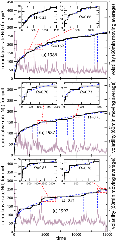
Figure 1: (Color online) Comparison between volatility and the cumulative rate $N(t)$ of volatilities (absolute 1 minute returns) larger than a threshold $q$. The plots show the 15,000 minutes (approximately two months) after the market crashes on (a) 11 September 1986, with $q=3$, (b) 19 October 1987, with $q=4$, and (c) 27 October 27 1997, with $q=4$. The volatility is displayed as a moving average over 60 minutes in order to suppress insignificant fluctuations. The insets show the self-similarity of the data set meaning that while the big crash in the beginning introduces a behavior following the Omori law, some of the aftershocks introduce again a similar behavior on a smaller scale.

II Omori law on different scales

Lillo and Mantegna Li+03 showed that the Omori law Omori1894 for earthquakes also holds after crashes of large magnitude in financial markets, so that the rate $n(t)$ of events with volatility larger than a given threshold $q$ decays as a power law

$$n(t)=kt^{-\Omega}\ \ ,$$ (1)

where $\Omega$ is around 1 for large $q$ and $k$ is a parameter characterizing the amplitude of the rate $n(t)$. For estimating the parameter $k$ and the exponent $\Omega$, we use the cumulative number $N(t)$ of events larger than $q$, given by

$$N(t)=\int_{0}^{t}n(t^{\prime})dt^{\prime}=k\frac{1}{1-\Omega}t^{1-\Omega}\ \ .$$ (2)

We study the Omori law on different time scales. Fig. 1 shows the cumulative rate $N(t)$ above (a) $q=3$ and (b,c) $q=4$ compared to the volatility in time periods following three significant market crashes in (a) 1986, (b) 1987, and (c) 1997. The volatility is smoothed by a moving average over 60 minutes in order to remove insignificant fluctuations. The large shock in the beginning of the time interval is followed by aftershocks, which induces an Omori-like behaviour of $N(t)$ (Omori process), shown by the dashed lines representing a power law fit. However, as seen in Fig. 1 (see insets) many of these aftershocks seem to behave like “real” crashes with their own aftershocks (subcrashes), but on a smaller scale (shown by vertical lines). The insets show that a closer look into many of these subcrashes reveals a similar pattern as the Omori law on large scales. The exponent $\Omega$ is often smaller after smaller crashes, which is consistent with the finding that the power law decay of the volatility after smaller shocks has a smaller exponent than after large crashes Sornette03 . Below we explore the possibility that the self-similarity of the volatility (where the Omori law is present on different scales) is directly related to the memory.

III Return interval memory after crashes and subcrashes

In order to explore the memory effects of the Omori law, we first analyze time periods after very large market crashes. Specifically, we study the memory in the volatility return intervals, which form a sequence of time intervals $\tau(t)$ between two consecutive events with volatilities larger than a given threshold $q$ Yam+05 ; Wang+06 ; Vodenska06 ; Wang++06 . We next show that the influence of the Omori law on $\tau(t)$ can be estimated by comparing the original $\tau(t)$ with a detrended time series $\tilde{\tau}(t)$ which is independent of the market crash. We fit the cumulative rate $N(t)$ in the period after a market crash with a power law according to Eq. (2), thus obtaining the parameter $k$ and the exponent $\Omega$ for the rate $n(t)$ Li+03 . Using $n(t)$, we can detrend the return interval time series $\tau(t)$ by rescaling by $n(t)$ Corral04

$$\tilde{\tau}(t)=\tau(t)n(t)\ \ .$$ (3)

The rational for this detrending is the following: immediately after the crash we have a large rate $n(t)$ of high volatilities so that the return intervals $\tau(t)$ are very short. Later, the rate of high volatilites becomes small while the return intervals get large. According to Eq. (3), high (low) rates and small (large) return intervals cancel each other so that $\tilde{\tau}(t)$ is detrended and thus independent of the existence of the crash, since the trend caused by the crash is no longer present.

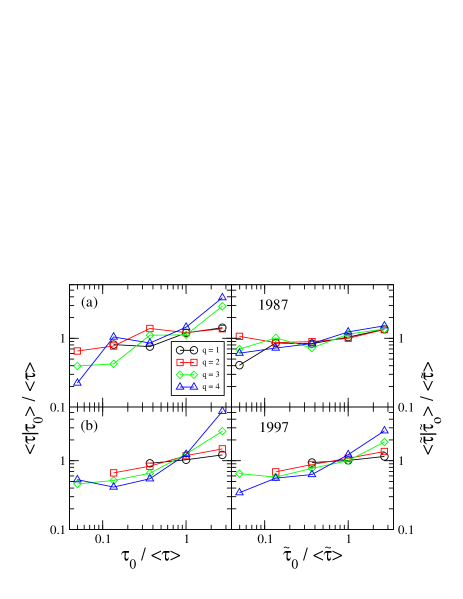
Figure 2: (Color online) Memory in volatility return intervals for different thresholds before (left column) and after (right column) detrending the time series according to Eq. (3). The analysis is shown for (a) the S&P500 index in the two months after the crash on 19 October 1987 and (b) an index calculated from the 100 most frequently traded stocks from the TAQ data base after the crash of 27 October 1997. Removing the Omori law reduces the memory in the data sets, but some memory still exists.

The relation between the Omori law and the short-term memory in the return interval time series can be studied by analyzing the conditional expectation value $\left<\tau(t)|{\tau_{0}}\right>$ of the return interval series $\tau(t)$ conditioned on the previous return interval $\tau_{0}$ Yam+05 ; Wang+06 , for both the original return intervals $\tau(t)$ and the detrended time series $\tilde{\tau}(t)$. In Fig. 2 (left column), $\left<\tau(t)|{\tau_{0}}\right>$ is plotted against $\tau_{0}$. Both quantities are normalized by the average return interval $\left<\tau\right>$, for return intervals after the crashes in (a) October 1987 and (b) October 1997. The deviations from a horizontal line at 1 for all thresholds show memory: large (small) values of $\tau_{0}$ are more likely to be followed by large (small) values of $\tau(t)$. The slopes of the curves for the detrended time series $\tilde{\tau}$ are significantly less steep (right column), indicating that detrending the Omori law from the time series significantly reduces the memory, but some of the memory still remains, which might be due to the Omori process still present on smaller scales (see Fig. 1).

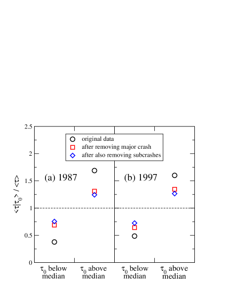
Figure 3: (Color online) Memory in volatility return intervals for threshold $q=3$ for (a) the S&P500 index in the two months after the crash on 19 October 1987 and (b) for an index calculated from the 100 most frequently traded stocks from the TAQ data base after the crash of 27 October 1997. The conditional expectation value $\left<\tau|\tau_{0}\right>/\left<\tau\right>$ conditioned on the previous return interval $\tau_{0}$ is smaller than 1 if $\tau_{0}$ is below the median while $\left<\tau|\tau_{0}\right>/\left<\tau\right>>1$ if $\tau_{0}$ is above the median, indicating the memory in the records (circles). The effect gradually weakens upon detrending the time series by removing the influence of the major crash (squares) and even further when removing some subcrashes (diamonds).

In addition to the effect of the major crash, we can also analyze the influence of Omori processes after subcrashes on smaller scales. To this end, we further detrend the time series by removing some subcrashes and test whether the memory is further reduced. After identifying the subcrashes, note2 we detrend the return intervals $\tau(t)$ by removing the Omori process due to the major crash as well as the Omori processes induced by the subcrashes. To this end, we estimate the parameters $k$ and $\Omega$ in Eq. (1) for the rate $n(t)$ after the major crash as well as for the rate $n_{s}(t)$ in the 1000 minutes following each subcrash (or the time to the next subcrash, if smaller). Note that $n_{s}(t)$ is calculated from the detrended return intervals $\tilde{\tau}(t)$. Then, the double detrended return interval time series is given by

$$\tilde{\tilde{\tau}}(t)=\left\{\begin{array}[]{ccc}n_{s}(t)\tilde{\tau}(t)&\mbox{in time following a subcrash}\\ \tilde{\tau}(t)&\mbox{otherwise.}\end{array}\right.$$ (4)

In order to improve the statistics for testing the effect of removing also subcrashes on the memory, we plot in Fig. 3 the conditional expectation value $\left<\tau|\tau_{0}\right>/\left<\tau\right>$ for only two $\tau_{0}$ intervals: $\tau_{0}$ below and $\tau_{0}$ above the median of $\tau$. We see in Fig. 3 that when $\tau_{0}$ is below the median, $\left<\tau|\tau_{0}\right>/\left<\tau\right><1$, while $\left<\tau|\tau_{0}\right>/\left<\tau\right>>1$ for $\tau_{0}$ above the median. This indicates the memory in the records, and also shows that the memory in the original records (circles) gradually weakens upon detrending the time series by removing the influence of the major crash (squares) and further weakens when also some subcrashes are removed (diamonds). Hence, not only a large market crash but also smaller subcrashes contribute to the memory in return intervals.

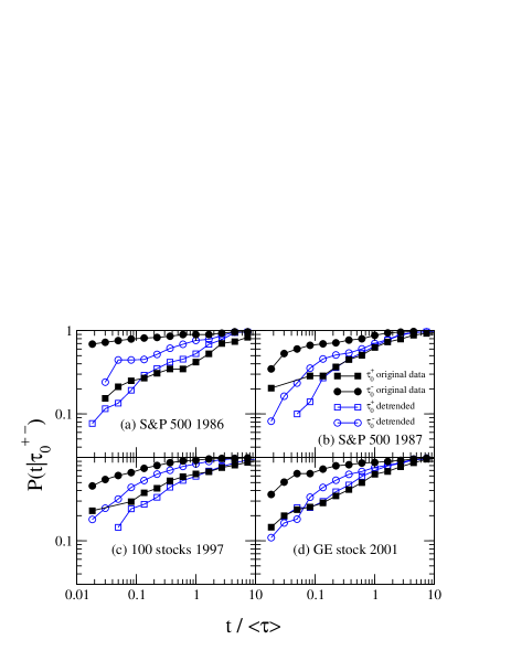
Figure 4: (Color online) Probability $P(t|\tau_{0})$ that after a return interval $\tau_{0}$ the next volatility larger than a threshold $q=4$ ($q=3$ in (d)) occurs within time $t$. Here, $\tau_{0}$ belongs to either the 25% smallest values ($\tau_{0}^{-}$, circles) or the 25% largest values ($\tau_{0}^{+}$, squares) of $\tau$. The memory in the original time series (filled symbols) is reduced by detrending according to Eq. (3) (open symbols), but some of the memory still remains. The results are shown for (a) the S&P500 index after a crash on 11 September 1986, (b) the S&P500 index after the crash on 19 October 1987, (c) an index created from the 100 most frequently traded stocks from the TAQ database after the crash on 27 October 1997 and (d) GE stock after 11 September 2001.

To further investigate the effect of removing the memory induced by aftershocks, we analyze the probability $P(t)$ that after an event larger than a certain volatility $q$ the next volatility larger than $q$ appears within a time $t$ Bunde05 ; Livina05 ; Vodenska06 . In order to study the memory, we plot the conditional probability $P(t|\tau_{0})$ for different values of the preceding return interval $\tau_{0}$. Fig. 4 shows $P(t|\tau_{0})$ for $q=2$ under the condition that the preceding return interval $\tau_{0}^{-}$ belongs to the the smallest 25% of the return intervals or that the preceding return interval $\tau_{0}^{+}$ belongs to the largest 25%. The memory in the time series leads to a splitting of the curves because after larger return intervals (squares) the time to the next volatility above $q$ is usually large, while it is short after small return intervals (circles). After detrending the time series the curves get closer, indicating a reduced memory, but also here some memory still remains.

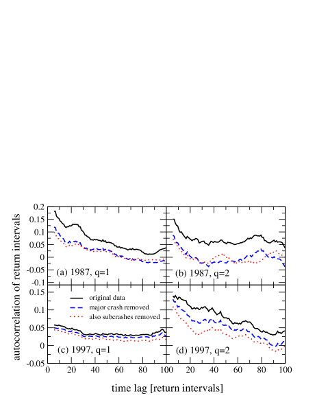
Figure 5: (Color online) Autocorrelation function of the return interval time series for threshold (a,c) $q=1$ and (b,d) $q=2$. The first row (a,b) shows results from the S&P500 index in the three months after the market crash on October 19, 1987, while the second row (c,d) results from an index created from the 100 most frequently traded stocks from the TAQ database after the crash on 27 October 1997. The Omori law due to the market crash (original data, solid lines) induces correlations leading to an offset in the autocorrelation function which is removed in the detrended $\tilde{\tau}$ (dashed lines), but the data still shows some long-term correlations even after removing the influence of the Omori law. However, after further detrending with respect to some subcrashes (dotted line), the autocorrelation is further reduced. All lines are smoothed by a moving average over 10 return intervals.

To test the long-term memory effects of the Omori process on the volatility return intervals we study the autocorrelation function shown in Fig. 5 for return intervals after the market crashes in 1987 and 1997 for two different thresholds $q=1$ and $q=2$. For both thresholds, we see that there exists a significant correlation even between return intervals 100 steps apart, which corresponds to approximately 2 to 5 days in 1987 (0.5 to 2 days in 1997) since the average return intervals are $\left<\tau(q=1)\right>=6.33$ min and $\left<\tau(q=2)\right>=17.4$ min in 1987 and $\left<\tau(q=1)\right>=2.47$ min and $\left<\tau(q=2)\right>=7.66$ min in 1997. If we now remove the effect of the Omori process due to the market crash by detrending according to Eq. (3), the memory in the detrended sequence $\tilde{\tau}$ is reduced significantly, as we see in the dashed curves of Fig. 5. The dotted lines show that removing also the influence of some subcrashes according to Eq. (4) further reduces the memory.

So far, we showed indications that within the time period after a big crash there might exist smaller crashes that behave in a similar way. The question arises whether such subcrashes are only typical after a big crash or whether they appear in all time periods independent of the existence of a big crash. To test this, we analyze if Omori processes exist also for smaller crashes. We study 22 crashes of sizes between 11 and 16 standard deviations in the S&P500 time series from 1984 to 1989. These crashes are considerably smaller than the huge crashes of more than 30 standard deviations in a 1 minute interval studied above. We analyze the cumulative rate $N(t)$ in the 1000 trading minutes following these smaller crashes. In order to make different crashes comparable irrespective of the current trading activity, we normalize the cumulative rate $N(t)$ by $N(1000)$. Fig. 6 shows this normalized rate $N(t)/N(1000)$ averaged over all aftershock periods note3 . For different thresholds $q$, $N(t)/N(1000)$ can be fit with a power law, Eq. (2). The exponent $\Omega$ increases with the threshold, but is generally smaller than the exponents found after very large shocks. Our results for the rate decay are analogous to volatility studies Sornette03 ; Zawadowski04 where the exponent characterizing the volatility decay depends on the magnitude of the shock Sornette03 . These results indicate that relatively small crashes have similar Omori processes which may lead to memory effects.

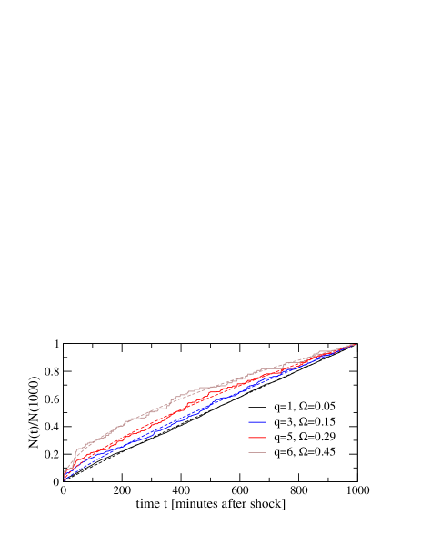
Figure 6: (Color online) Cumulative rate $N(t)$ of events larger than a threshold $q$ averaged over the 1000 minutes after 22 shocks between $11\sigma$ and $16\sigma$ in the S&P500 one minute time series of the years 1984 to 1989. The data for each shock is normalized by $N(1000)$ in order to make different shocks comparable irrespective of the current trading activity. The cumulative rate can be well fitted by a power law according to Eq. (2). The exponent grows from $\Omega=0.05$ to $\Omega=0.45$ for $q=1\dots 6$.

IV Memory in Volatility after crashes and subcrashes

In the previous sections, we showed that the memory in return intervals decreases when we remove effects due to Omori processes. Since the studied return intervals $\tau(t)$ are derived from the volatility time series $v(t)$, it would be interesting to test whether the memory in $v(t)$ is also affected by Omori processes. Thus, we next analyze the memory in the volatility time series directly. It is known that a market crash induces a power law decay of the approximate form

$$v_{PL}(t)\equiv v_{0}t^{-\beta}$$ (5)

with an exponent $\beta\approx 0.2-0.3$ Li+03 ; Sornette03 . In order to study the memory induced by this decay, we compare the original time series $v(t)$ to a detrended one

$$\tilde{v}(t)\equiv\frac{v(t)}{v_{PL}(t)}$$ (6)

so that $\tilde{v}(t)$ does not depend on the market crash.

We use second order detrended fluctuation analysis (DFA2) Peng94 ; Bunde00 to study the long-term memory in the volatility Liu99 ; Wood85 ; Harris86 ; Admati88 ; Schwert89 ; Chan91 ; Bollerslev92 ; Gallant92 ; Baron92 ; Ding93 ; Dacorogna93 ; Pagan96 ; Granger96 ; Liu97 ; Cont98 ; Pasquini99 ; Plerou2001 . In DFA2, the deviations $F(s)$ (root mean square fluctuations) from a second degree polynomial fit of the profile

$$y(t)=\sum_{t^{\prime}=0}^{t}v(t^{\prime})$$ (7)

as a function of different scales $s$ (time windows) reveal information about the memory. If $F(s)\sim s^{\alpha}$, the autocorrelation exponent $\gamma$ of the time series is related to the exponent $\alpha$ by $\alpha=1-\gamma/2$. For $\alpha>0.5$, the time series is long-range correlated, it is anti-correlated for $\alpha<0.5$, and $\alpha=0.5$ indicates no long-range correlations. Fig. 7 shows $\log(F(s)/s^{0.5})$ plotted against $\log s$ for 15,000 trading minutes after three different market crashes of 1986, 1987, and 1997. With no long-term correlations, the function would be constant, while a positive slope indicates long-term correlations. For all crashes, the original time series (circles) shows an increased slope on large time scales. After detrending according to Eq. (6) and replacing $v(t^{\prime})$ by $\tilde{v}(t^{\prime})$ in Eq. (7), the curve (squares) gets less steep, indicating a reduction of the memory (the curves are shifted so that they start at the same point).

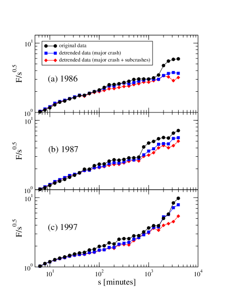
Figure 7: (Color online) Root mean square fluctuation $F(s)$ obtained by the second order DFA method (DFA2) for the volatility in the 15000 minutes following market crashes in (a) the S&P500 index on 11 September 1986 and (b) on 19 October 1987, as well as (c) the market crash on 27 October 1997 for an index created from TAQ-data for 100 stocks. $F(s)$ is divided by $s^{0.5}$ to clarify the deviation from uncorrelated data. Compared to the original volatility $v(t)$ (circles), the memory is reduced in the detrended records $\tilde{v}(t)$ (squares), and even further after also detrending some subcrashes in $\tilde{\tilde{v}}(t)$ (diamonds).

As described before, there are also subcrashes which may induce their own power law decay on a smaller scale – not only in the rate, but also in the volatility. In order to analyze the memory due to these subcrashes, we further detrend the time series and test whether the memory is reduced even further. To this end, we fit the detrended volatility $\tilde{v}(t)$ in the 1000 minutes following each subcrash (or the time to the next subcrash, if shorter) with a power law $\tilde{v}_{PL}$ according to Eq. (5). Then, we further detrend $\tilde{v}(t)$ in these regions using Eq. (6) for $\tilde{v}(t)$ instead of $v(t)$. The DFA2 curve for the double detrended time series $\tilde{\tilde{v}}(t)\equiv\tilde{v}/\tilde{v}_{PL}$ is shown in Fig. 7. The decrease in the slope shows that the memory is further reduced after removing the influence of the subcrashes. However, we clearly see that removing the trends induced by a market crash as well as subcrashes only slightly reduces the memory in the volatility on quite small scales ($s<60$ min).

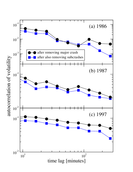
Figure 8: (Color online) Autocorrelation function of the volatility time series after detrending. Compared to the volatility time series after detrending the major crash (circles), detrending subcrashes (squares) further reduces the autocorrelations. The results are shown for (a) the S&P500 index after a crash on 11 September 1986, (b) the S&P500 index after the crash on 19 October 1987, (c) an index created from the 100 most frequently traded stocks from the TAQ database after the crash on 27 October 1997. The autocorrelation function of the original volatility time series is not shown because it is not meaningful as it is dominated by the influence of the market crash.

The effect of removing subcrashes on the long-term correlations of volatility is seen better in Fig. 8. Here, we compare the autocorrelation functions of the detrended volatility $\tilde{v}(t)$ and the double detrended volatility $\tilde{\tilde{v}}(t)$ after also removing subcrashes. It is seen that generally the autocorrelation of $\tilde{\tilde{v}}(t)$ is smaller than of $\tilde{v}(t)$, which indicates that the Omori processes after subcrashes also contain some memory.

V Discussion and conclusions

We find that the volatility exhibits some self-similar features, meaning that Omori processes exist not only on very large scales, but a similar behavior is also induced by less significant shocks in the aftershocks. After a large market crash, some of the aftershocks can be considered as subcrashes that initiate Omori processes on a smaller scale.

We ask the question whether this self-similarity can be responsible for the memory in volatility return intervals as well as in the memory of the volatility itself. Our results show that a significant amount of memory is induced by these crashes and subcrashes, which suggests that a large part of the memory in volatility might be due to Omori processes on different scales.

References

- (1) R. A. Wood, T. H. McInish, and J. K. Ord, J. Finance 40, 723 (1985).
- (2) L. Harris, J. Financ. Econ. 16, 99 (1986).
- (3) A. Admati and P. Pfleiderer, Rev. Financ. Stud. 1, 3 (1988).
- (4) G. W. Schwert, J. Finance 44, 1115 (1989).
- (5) K. Chan, K. C. Chan, and G. A. Karolyi, Rev. Financ. Stud. 4, 657 (1991).
- (6) T. Bollerslev, R. Y. Chou, and K. F. Kroner, J. Econometr. 52, 5 (1992).
- (7) A. R. Gallant, P. E. Rossi, and G. Tauchen, Rev. Financ. Stud. 5, 199 (1992).
- (8) B. Le Baron, J. Business 65, 199 (1992).
- (9) Z. Ding, C. W. J. Granger, and R. F. Engle, J. Empirical Finance 1, 83 (1993).
- (10) M. M. Dacorogna, U. A. Muller, R. J. Nagler, R. B. Olsen, and O. V. Pictet, J. Int. Money Finance 12, 413 (1993).
- (11) A. Pagan, J. Empirical Finance 3, 15 (1996).
- (12) C. W. J. Granger and Z. Ding, J. Econometr. 73, 61 (1996).
- (13) Y. Liu, P. Cizeau, M. Meyer, C.-K. Peng, and H. E. Stanley, Physica A 245, 437 (1997); P. Cizeau, Y. Liu, M. Meyer, C.-K. Peng, and H. E. Stanley, Physica A 245, 441 (1997).
- (14) R. Cont, Ph.D. thesis, Universite de Paris XI, 1998 (unpublished); see also e-print cond-mat/9705075.
- (15) M. Pasquini and M. Serva, Econ. Lett. 65, 275 (1999).
- (16) Y. Liu, P. Gopikrishnan, P. Cizeau, M. Meyer, C.-K. Peng, and H. E. Stanley, Phys. Rev. E 60, 1390 (1999).
- (17) V. Plerou, P. Gopikrishnan, X. Gabaix, L. A. N. Amaral, and H. E. Stanley, Quant. Finance 1, 262 (2001); V. Plerou, P. Gopikrishnan, and H. E. Stanley, Phys. Rev. E 71, 046131 (2005).
- (18) It has been known for some time that, qualitatively, there appears to be a “slow” Chan91 or “very slow” Schwert89 decay of the autocorrelation function of absolute returns. Later, attempts were made to quantify this slow decay. For example. Ding et al. Ding93 analyzed daily returns of the S&P500 index time series for a period of more than 60 years. They found that a power law fit of the autocorrelation function of the absolute return decreases too fast in the beginning (i.e. short time lags) but too slow for long time lags. Hence, they fit the data with a combination of an exponential function and a power law. Dacorogna et al. Dacorogna93 studied the autocorrelation of the absolute return in the foreign exchange market. Using four years of 20 minute returns of different exchange rates, they find that a hyperbolic curve (i.e. a power law) fits the data much better than an exponential curve. The power law exponent varies between 0.2 and 0.3 depending on the exchange rate. Moreover, they found that the decay becomes faster when considering very large time lags of more than 10 days. Liu et al. Liu97 ; Liu99 analyzed the 1 minute returns of the S&P500 index over a 13 year-period using detrended fluctuation analysis (DFA), and found that the autocorrelation of the absolute return exhibits a power law decay with two different exponents 0.31 (short time lags) and 0.9 (long time lags).
- (19) K. Yamasaki, L. Muchnik, S. Havlin, A. Bunde, and H. E. Stanley, Proc. Natl. Acad. Sci. 102, 9424 (2005).
- (20) F. Wang, K. Yamasaki, S. Havlin, and H. E. Stanley, Phys. Rev. E 73, 026117 (2006).
- (21) To properly identify subcrashes that can be removed from the records, we filter the time series with an appropriate criteria for each data set. For the S&P500 index time series, including the crashes from 1986 and 1987, we define a subcrash as an event where the 60 minute moving average of the 1 minute volatility exceeds 1 standard deviation (corresponding to a much larger 1 minute volatility burst). We also require at least 500 minutes to the next subcrash (events within 100 minutes are considered as the same subcrash). For the data from 1997, we analyze the 10 minute moving average, and a subcrash has to exceed 2.5 standard deviations. The other parameters are the same as for the S&P500 data.
- (22) I. Vodenska-Chitkushev, F. Wang, P. Weber, K. Yamasaki, S. Havlin, and H. E. Stanley, (preprint).
- (23) F. Wang, P. Weber, K. Yamasaki, S. Havlin, and H. E. Stanley, Eur. Phys. J. B (in press).
- (24) V. N. Livina, S. Havlin, and A. Bunde, Phys. Rev. Lett. 95, 208501 (2005).
- (25) A. Bunde, J. F. Eichner, S. Havlin, and J. W. Kantelhardt, Physica A 342, 308 (2004).
- (26) A. Bunde, J. F. Eichner, J. W. Kantelhardt, and S. Havlin, Phys. Rev. Lett. 94, 048701 (2005).
- (27) F. Lillo and R. N. Mantegna, Phys. Rev. E 68, 016119 (2003).
- (28) F. Omori, J. Coll. Sci. Imp. Univ. Tokyo 7, 111 (1894).
- (29) The average only includes crashes where the volatility exceeds the threshold at least 5 times during the studied time period of 1000 minutes. For e.g. , there are 11 crashes that satisfy this criteria.
- (30) D. Sornette, Y. Malevergne, and J. F. Muzy, Risk Magazine 16, 67 (2003).
- (31) A. G. Zawadowski, J. Kertesz, and G. Andor, Physica A 344, 221 (2004).
- (32) A. Corral, Phys. Rev. Lett. 92, 108501 (2004).
- (33) C.-K. Peng, S.V. Buldyrev, S. Havlin, M. Simons, H.E. Stanley, and A.L. Goldberger, Phys. Rev. E 49, 1685 (1994); C.-K. Peng, S. Havlin, H.E. Stanley, A.L. Goldberger, Chaos 5, 82 (1995).
- (34) A. Bunde, S. Havlin, J.W. Kantelhardt, T. Penzel, J.-H. Peter, and K. Voigt, Phys. Rev. Lett. 85, 3736 (2000); K. Hu, P. Ch. Ivanov, Z. Chen, P. Carpena, and H. E. Stanley, Phys. Rev. E 64, 011114 (2001); Z. Chen, P. Ch. Ivanov, K. Hu, and H. E. Stanley, Phys. Rev. E 65, 041107 (2002); Z. Chen, K. Hu, P. Carpena, P. Bernaola-Galvan, H. E. Stanley, and P. Ch. Ivanov, Phys. Rev. E 71, 011104 (2005); L. Xu, P. Ch. Ivanov, K. Hu, Z. Chen, A. Carbone, and H. E. Stanley, Phys. Rev. E 71, 051101 (2005).