Molecular configurations in a droplet detachment process of a complex liquid

Abstract

We studied the microscopic polymer conformations in the droplet detachment process of an elastic semi-dilute polyelectrolytic Xanthan solution by measuring the instantaneous birefringence. As in earlier studies, we observe the suppression of the finite time singularity of the pinch-off process and the occurrence of an elastic filament. Our microscopic measurements reveal that the relatively stiff Xanthan molecules are already significantly pre-stretched to about 90 $\%$ of their final extension at the moment the filament appears. At later stages of the detachment process, we find evidence of a concentration enhancement due to the elongational flow.

I Introduction

The addition of a tiny amount of polymer to a simple liquid alters the dynamics of a droplet detachment process dramatically. Instead of the finite time singularity of the minimum neck diameter [1], a cylindrical filament is formed and the shrinking dynamics can be slowed down by several decades[2, 3, 4, 5]. Despite the technological relevance of the droplet forming process of complex liquids that reaches from plotting of DNA-microarrays to food processing, only little is known on the underlying physical mechanisms. Besides the complexity of the problem and the lack of a universally applicable constitutive equation for complex liquids, there exist no microscopic data on the molecular conformation in such a flow. It is the goal of this study to close this gap.

Earlier experimental studies on the droplet detachment process of complex liquids were limited to the analysis of macroscopic quantities like the determination of the shape of the thinning filament. These can be compared with theoretical analysis on capillary break-up based on phenomenological polymer models like e.g. the Oldryd-B or models that follow from kinetic theory like FENE-P [6]. But for a true comparison with microscopic models, the dynamics of the polymers on the molecular level must be measured. Birefringence is a typical tool for such investigations [7], and we use a high speed set-up capable of capturing dynamics on the time scale of milliseconds to study both the microscopic conformation and the macroscopic flow response in the elastic thread simultaneously.

II Sample characterization

The polymeric system of our study, Xanthan (Sigma-Aldrich), was chosen because of its high optical anisotropy. The molecular weight of t our polymer $m$ is vaguely specified by the distributor with “$m=2\times 10^{6}$ amu or more“. Xanthan shows a pronounced shear thinning and biological digestibility and, for both reasons, it is widely used in the food, pharmaceutical, oil, and cosmetic industries. The ordered molecule exists in solution as a semi rigid helix with a persistence length of 120 nm. It undergoes a conformational transition to a disordered flexible coil only above a temperature of $50^{\circ}C$ [8, 9].

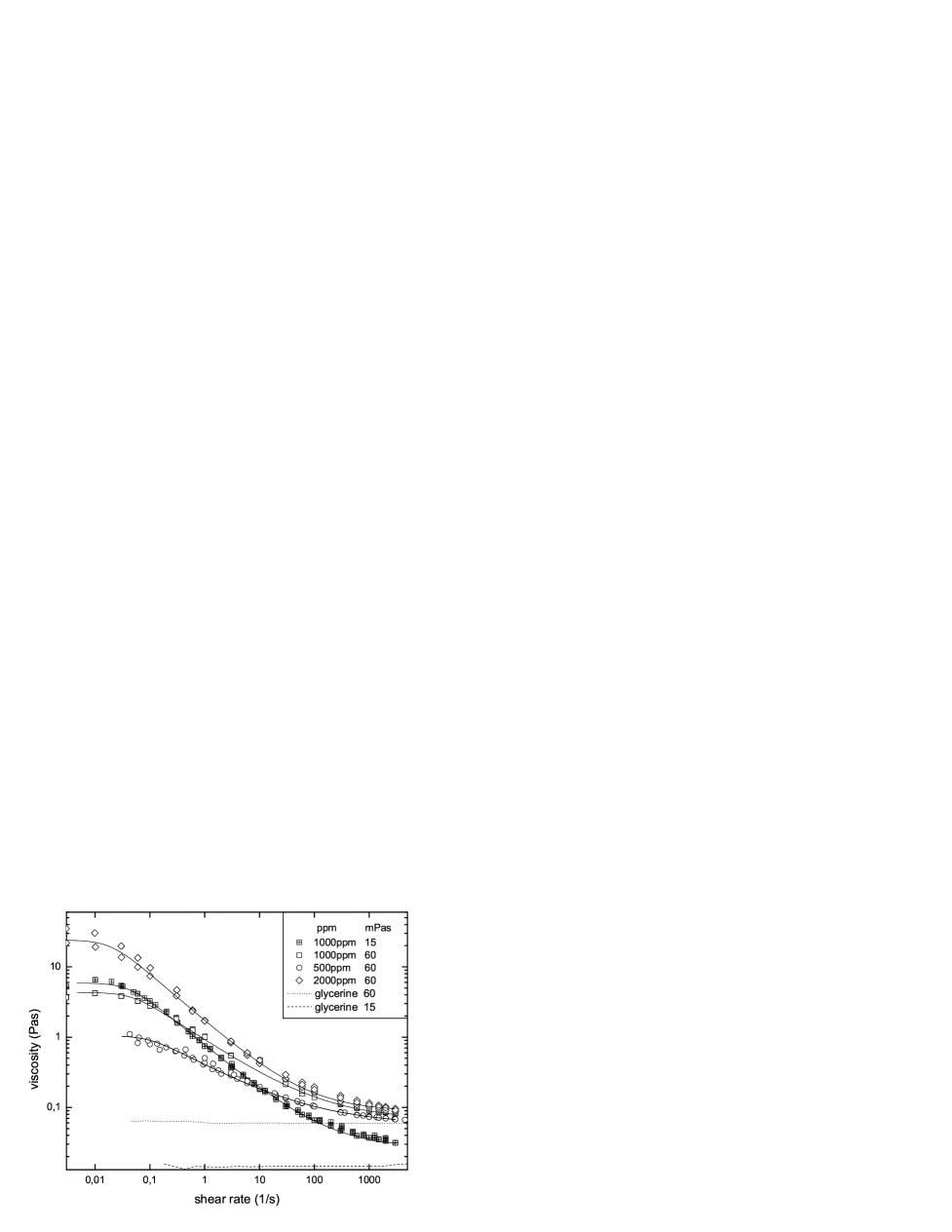
FIG. 1.: Stationary viscosities from shear rate and stress controlled measurements. Not all experiments and data points are shown. The lines are approximations by the Carreau model.

Our sample solutions were prepared with weight concentrations $c_{p}$ in the semi-dilute regime from $250ppm<c_{p}<2000ppm$, mostly dissolved in $80/20$ weight$\%$ glycerol-water as a solvent with a viscosity of $\eta_{solv}=60mPas$. We also used different glycerol-water weight ratios resulting in solvent viscosities down to $\eta_{solv}=2mPas$ only to allow for a better determination of the molecular weight of our sample by fitting our extensional rheological data. The polymer concentrations where chosen to obtain a sufficiently high birefringence but still to be significantly below concentrations at which spontaneous lyotropic ordering is expected in equilibrium ($c_{p}>5000ppm$) [8]. Standard rheological measurements, using a cone plate geometry on a standard Rheometer (Haake Mars, Thermo Electron, Germany) were performed to characterize the shear thinning behavior (fig. 1) of our samples. Stationary experiments controlling either shear rate or tension were repeated several times for several samples in a cone plate geometry with an angle of $0.5^{\circ}$ and a diameter of $60mm$. Depending on the experimental deviations an average of between 6 and 10 measurements is shown. The solutions show a pronounced shear thinning, as to be expected for relatively stiff molecules approaching a stationary value slightly enhanced compared to the pure Newtonian solvent according to the polymer concentration. The data have been approximated using the Carreau model [11] and the results are in reasonable agreement with ref. [10] if one takes our higher solvent viscosities into account. The characteristic relaxation times of the fits range from about $10s$ for $500ppm$ and $20s$ for $1000ppm$ to about $50s$ for the $2000ppm$ solution. These time scales give a measure for the rotational diffusion time of our molecules and must be compared with the elongational rates in our droplet experiments.

For the later discussion of our elongational viscosity measurements we would like especially to point out that the 1000 ppm samples with different solvent viscosities show similar zero shear rate viscosities, and the differences only become obvious at high shear rates.

III Experimental setup

The experimental setup is sketched in fig. 2A. The polymer solutions are quasistatically driven through a nozzle of $d=2mm$ diameter by a syringe pump. At a distance of $D=7cm$ below the nozzle, a plate is mounted in order to omit gravitational effects, and to stabilize the filament against air currents. All measurements have been performed at room temperature ($25^{\circ}C$). The retardation $\delta$ is measured using an optical train consisting of an 18mW HeNe Laser (JDS Uniphase), a Polarizer P, a Photo Elastic Modulator PEM (Hinds Instruments), the sample liquid, an Analyzer A, a bright field lens system L1 and L2, and a photo diode PD connected to two Lock-Ins (Stanford Research). The polarizer is fixed at an angle of $45^{\circ}$ relative to the photo elastic modulator which allows for a Lock-In technique for the detection of the retardation signal. The bright field lens system (fig. 2B) in front of the detector prevents any light that has not crossed the filament (fig. 3)) from reaching the detector by blocking the parallel components with a mask M in the focal point of lens L1. The lens L2 collects the light that is diffused by the cylindrical filament into the detector [12]. To calculate the birefringence $\Delta n=\delta h(t)/(2\pi\lambda)$ (with $\lambda=633nm$ as the HeNe laser wavelength) from the retardation signal the instantaneous thickness $h(t)$ of the filament must be known. The thinning process of the filament diameter $h(t)$ is measured at 500 frames per second with a high speed CCD-camera (encore mac PCI 1000S) that is placed perpendicular to the optical train. The camera is equipped with a 2 times magnification objective and the image capturing is synchronized to the data collection of the two Lock-In s. From fig. 3 it becomes obvious that, for geometric reasons, it is impossible to measure birefringence before the droplet has completely passed the light beam and the temporal exponentially thinning filament is present. This is the moment when our measurements start.

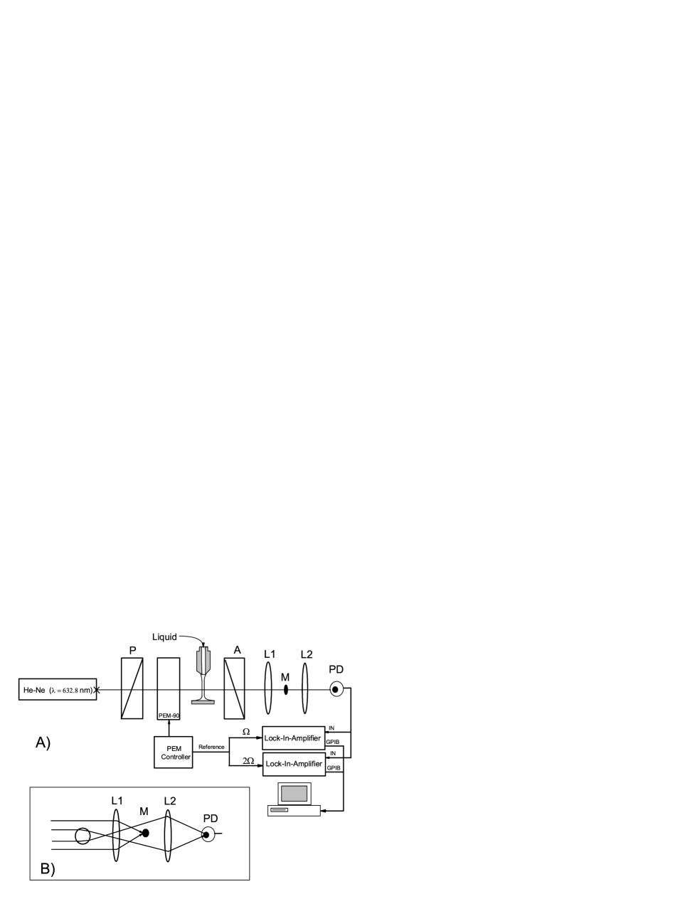
FIG. 2.: The experimental setup. See text for further explanation.

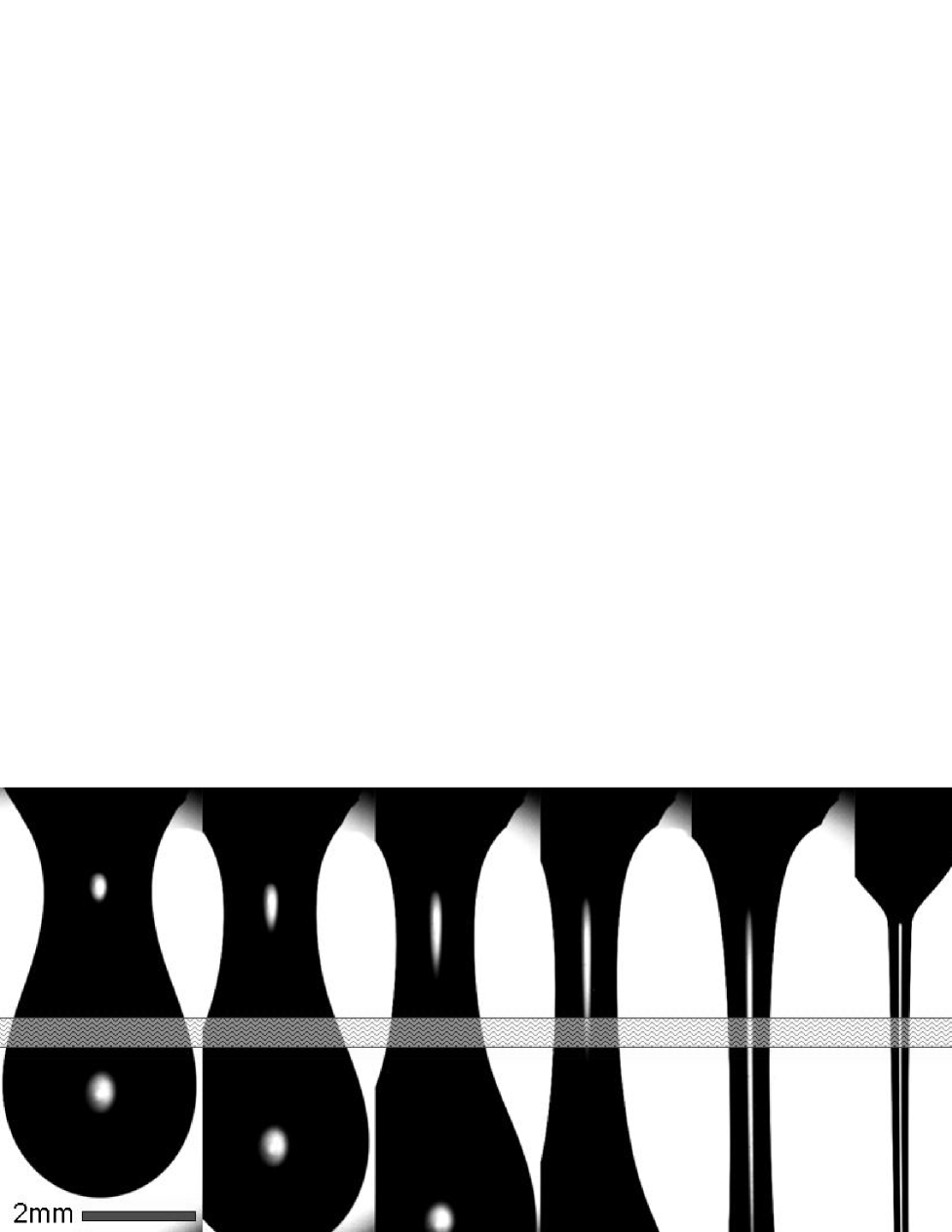
FIG. 3.: Photographs of the droplet detachment process of a 2000 ppm Xanthane solution ($\eta_{solv}$=60mPas) taken every 0.1s indicating, schematically, the laser beam positioned close to the neck and in a region as cylindrical as possible throughout the measurement.

IV Experimental results

A Macroscopic measurements

Different regimes can be distinguished analysing the temporal behavior of the neck diameter $h(t)$ in the droplet detachment process of a polymer solution. First, it follows an exponential law that is well described by the Rayleigh instability of Newtonian liquids [13, 14]. Then it might pass into the self similar regimes that describe the break-up of Newtonian liquids [15] until the polymers intervene the flow abruptly and a filament is formed which, again, thins very slowly and exponentially with time [16].

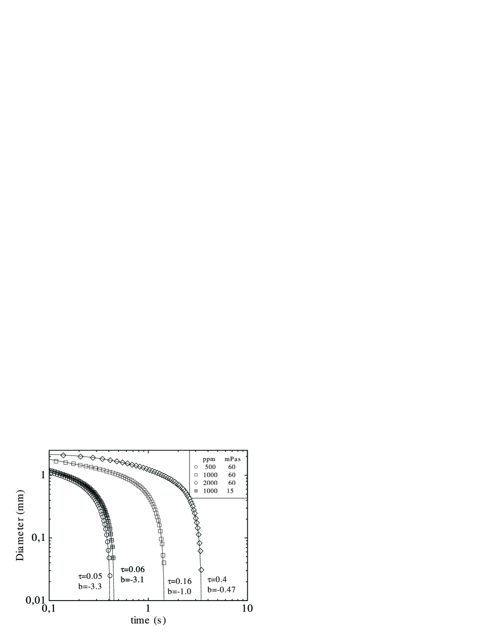
FIG. 4.: Filament diameter h(t) for different polymer concentrations and solvent viscosities. The parameters refer to eq. 1. Not all data points are shown.

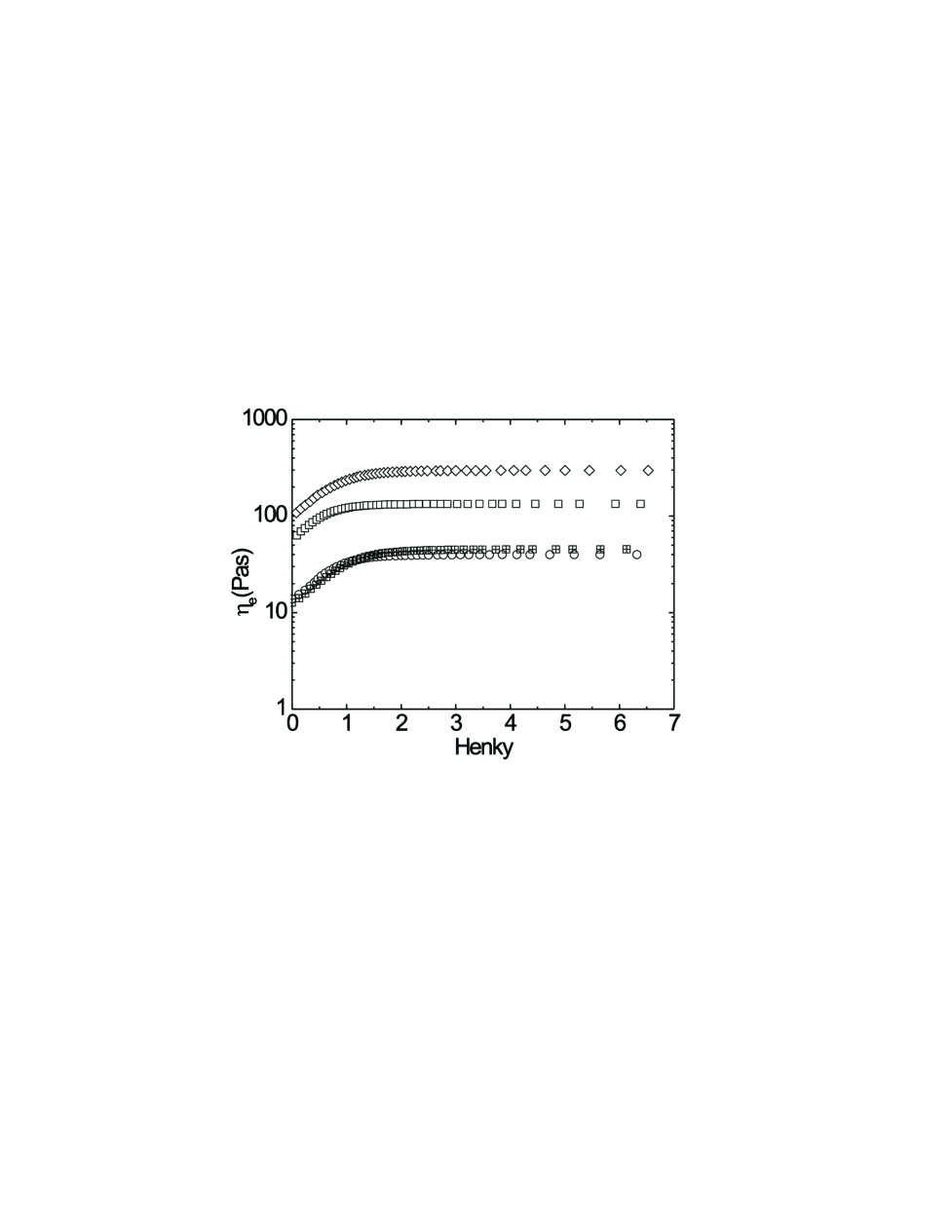
FIG. 5.: The apparent elongational viscosity for the same set of data as in fig. 4

Figure 4 shows the filament thickness $h(t)$ extracted from the video images that start at the moment when the filament is formed. More viscous solvents or higher polymer concentrations lead to a slower dynamic that differs by more than an order of magnitude. However, at first all runs show the same exponential thinning behavior, followed by a linear regime, and the data can be approximated by the expression

$$h(t)=exp(-t/\tau)-bt+y_{o}.$$ (1)

The formation of the cylindrical filament occurs due to the high resistance of the polymers to elongational flow and this resistance is macroscopically quantified by the elongational viscosity $\eta_{e}$. The same form of equation 1 has been used to fit data from extensional rheology measurements (both capillary break up and filament stretching devices[17]). Its physical meaning is that first the polymer molecules are uncoiled by the flow and the dynamic is governed purely by elastic effects. Once the polymers are stretched, a steady state is reached which leads to the linear dynamic. From $h(t)$ one can calculate the corresponding elongational rates $\dot{\epsilon}=\partial_{t}h(t)/h(t)$. These have to be compared with characteristic relaxation times. The microscopic polymer rotational diffusion has been estimated by the time constants from the standard rheological measurements to be at least $\lambda>10s$ and the appropriate ratio is given by the Weissenberg number which is always found to be very large $Wi=\lambda\dot{\epsilon}>100$ in our experiments. This means that the polymer molecules in the droplet detachment process do not experience a force field that is comparable to the Brownian forces and time scales, but are affected by a violent flow and stretched and oriented in a deterministic manner. Nevertheless, the elongational rates and the Weissenberg numbers are practically constant in the regime of exponential thinning. They diverge, though, when the linear thinning behavior sets in.

The $h(t)$ data can also be used directly to calculate the apparent elongational viscosity by equating the capillary pressure with the elastic stresses [3, 4, 17]:

$$\eta_{e}(t)=\frac{2\sigma}{\dot{\epsilon}h(t)}$$ (2)

This approach is a simplification because it neglects gravitational or nonlinear elastic effects, but it is commonly used to extract the elongational viscosity from capillary break up experiments. A common quantity representing the stress- and stretching history of the fluid, and thereby the polymers, is the Henky strain given by $\zeta=\int\dot{\epsilon}dt$. The corresponding elongational viscosity data in fig. 5 first show an exponential increase of the apparent elongational viscosity followed by a steady state value for strains $\zeta\geq 1.5$. The observation of the plateau value at strains that much smaller compared to earlier work [4, 17, 18] is a consequence of the relative stiffness of the Xanthan molecule and the pre-stretching before the occurrence of the filament. This is also indicated by the elevated elongational viscosity at $\zeta=0$. If the filament would start to be formed with the polymers at rest one would expect the elongational viscosity to grow from the Newtonian value of the so called Trouton ratio $\eta_{e}/\eta_{s}=3$. When $\eta_{e}$ reaches the plateau value the thinning dynamic becomes linear and the elongational rate $\dot{\epsilon}$ diverges, indicating that $\eta_{e}$ is independent of the elongational rate as predicted by rigid rod models as well as elastic models for $Wi>>1$ [19]. The measured elongational viscosities are in reasonable agreement with data from studies with opposing nozzles [20], fiber spinning devices [21], or values obtained by analyzing contraction flow [22]

For our birefringence study we needed an estimate for the molecular weight of our sample and we used Batchelors formula [Batchelor] for the elongational viscosity of semidiluted rigid rods to fit our data. Fluorescence microscopy studies on DNA show that at steady state for Henky strains $\zeta\geq 1.5$ the molecules are extended to a maximum hydrodynamic length $\ell$ that is more than $80\%$ of their contour length [23], and the relatively stiff Xanthan molecules are mostly well approximated as rigid rods. In order to allow for a robust fitting procedure for the determination of the two free parameters molecular weight $m$ and polymer length $\ell$ we varied both the polymer concentration and the solvent viscosity. As expected we found the elongational viscosity to always be proportional to the solvent viscosity (see fig. 5). With our two independent sets of data, we performed the fit with Batchelors formula for semidiluted solutions of rigid rods (fig. 6)

$$\eta_{e}=3\eta_{solv}+\frac{\frac{2}{3}\eta_{solv}\Phi(\ell/d)^{2}}{ln(2\ell/d)-ln(1+2\sqrt{\Phi/\pi}\ell/d)-1.5}$$ (3)

$\Phi$ is the particle volume fraction and, for the width of the polymer, we took the literature value of $d=2nm$. The fit yields $\ell=4.5\mu m$ and $m=2.5$ Mamu. This ratio of molecular weight and length is in very good agreement with e.g. the results from a contraction flow study by [22], but differs by a factor of two from values obtained by light scattering [20]. The number of Kuhn steps of our sample is about $40$, a value that is 10 times smaller than that of $\lambda$-DNA which has been used in a previous study where no steady state of the elongational viscosity had been observed [18].

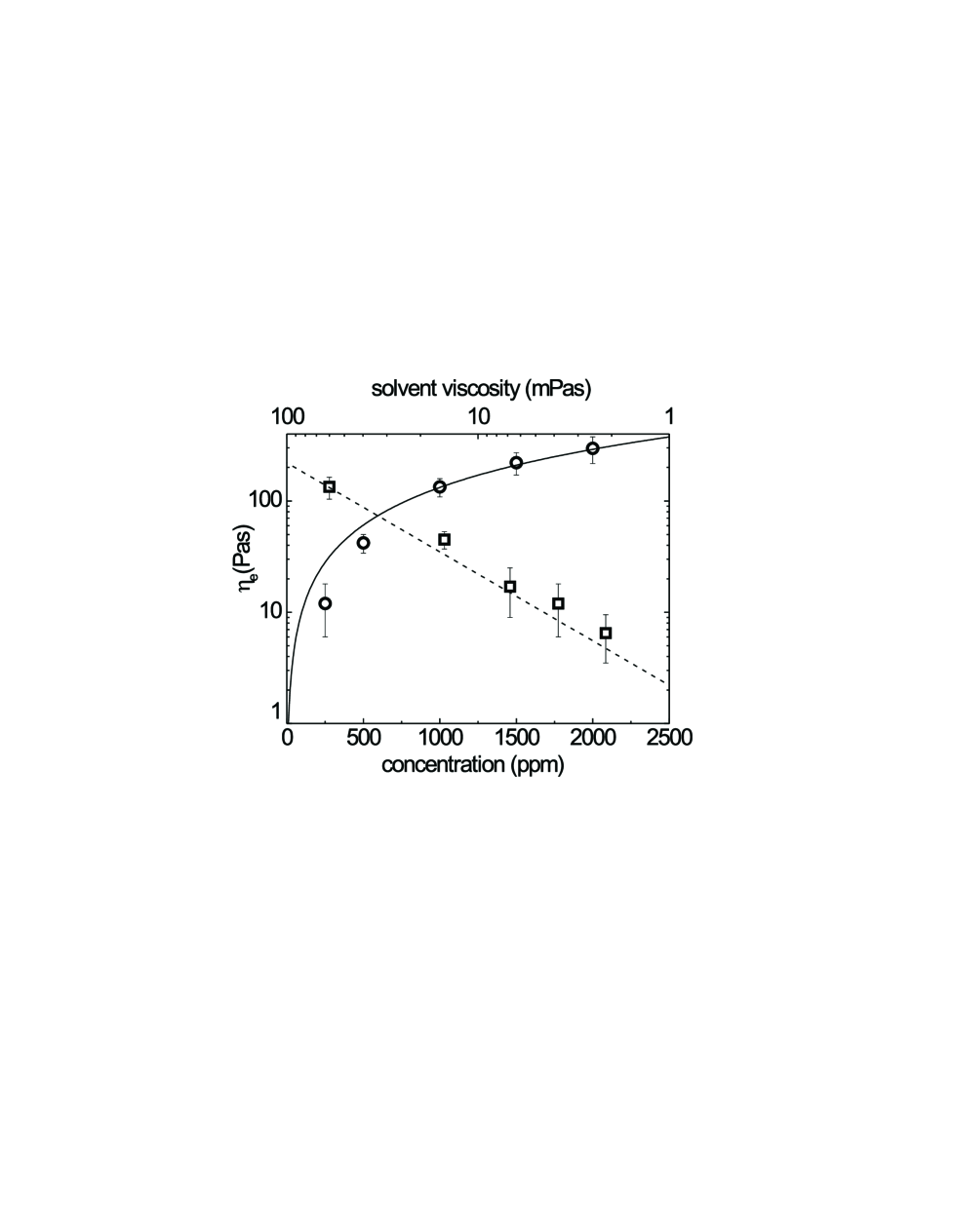
FIG. 6.: The elongational viscosity for different solvent viscosities (squares) and polymer concentrations (circles). The continuous and the dashed lines show the theoretical values according to Batchelors formula for semidiluted rigid rods.

B Birefringence measurements

We can now turn to the microscopic study of the conformation of the macromolecules by means of the birefringence measurements. An elaborate introduction in optical flow rheometry is given in [7]. In our unidirectional stretching geometry with the flow along the direction of gravity, we can assume transverse isotropy for polarizability and segmental order of the single units of the macromolecules. Therefore, the birefringence signal $\Delta N$ is proportional to the segmental order of the polymers and to their concentration

$$\Delta N=\frac{2\pi}{nm}\Delta\alpha_{0}c_{p}N_{a}\frac{1}{2}<3\cos^{2}\theta-1>$$ (4)

where n is the average refractive index, $N_{a}$ the Avogadro number and $\theta$ the orientation angle of the polymer segments to the direction of extension. By knowledge of the maximum birefringence signal $\Delta N_{max}$ at maximum extension and alignment of the polymers, the mean fractional extension of our polymers is then $x/\ell=\sqrt{(2\Delta N/\Delta N_{max}+1)/3}$ because, on a microscopic scale, a variety of different configurations will certainly be present [23].

The negligence of different configuration types like, e.g., dumbbell or hairpin, leads to a certain overestimate of the fractional extension and our calculation looses its accuracy for coiled states. The correctness of the formula improves, though, increasing degree of orientational order and is a good approximation for large fractional extensions of the stretched polymers.

To test the reliability of our method we performed several runs at different polymer concentrations, and the birefringence signal was always roughly proportional to the concentration (fig. 7b). The robustness and selectivity of our method becomes clear if one compares the data of the solution with $500ppm$ of polymer and $\eta_{solvent}=60mPas$ with the solution with $1000ppm$ of polymer and $\eta_{solvent}=15mPas$. Both data sets practically lead to the same flow (fig. 4) but, exceeding the capabilities of simple extensional rheometry, the birefringence signal is sensitive to the differences in concentration. This shows how important the microscopic measurements are if one wants to qualify theoretical predictions that are based on kinetic models.

The measurements of the birefringence in our setup are restricted to the time $t_{c}$ after the filament is formed because optical abberations make it impossible to measure it at earlier stages of the pinching process. Even if the origin of the Hencky strain is not influenced much by this limitation, as most of the strain is accumulated at the final stages of the experiment, our data reveal that the polymers have a significant (flow and strain) history when our measurements start. Assuming that the polymers are completely stretched when elastic effects are no longer observable for $\zeta\geq 1.5$, we can calculate the maximum birefringence per polymer concentration $\Delta N_{max}/c_{p}=8\times 10^{-2}g^{-1}cm^{3}$. This is comparable to the value for fully elongated $\lambda$ DNA of $\Delta N_{max}/c_{p}=5.1\times 10^{-2}g^{-1}cm^{3}$ [24], but a decade larger than values obtained for Xanthan in shear flow [25] and in transient electric birefringence measurements [26].

The corresponding maximum birefringence of the $c_{p}\leq 1000ppm$ solutions is only $~{}30\%$ larger than at $\zeta=0$. This would correspond to a fractional polymer extension $x/\ell=0.9$ at $\zeta=0$, indicating that stiff polymers like Xanthan are almost completely aligned and stretched when the filament occurs. The uncoiling process in the range $0<\zeta<1.5$ correlates with an elastic, exponential filament thinning dynamic and a monotonic increase of the birefringence signal.

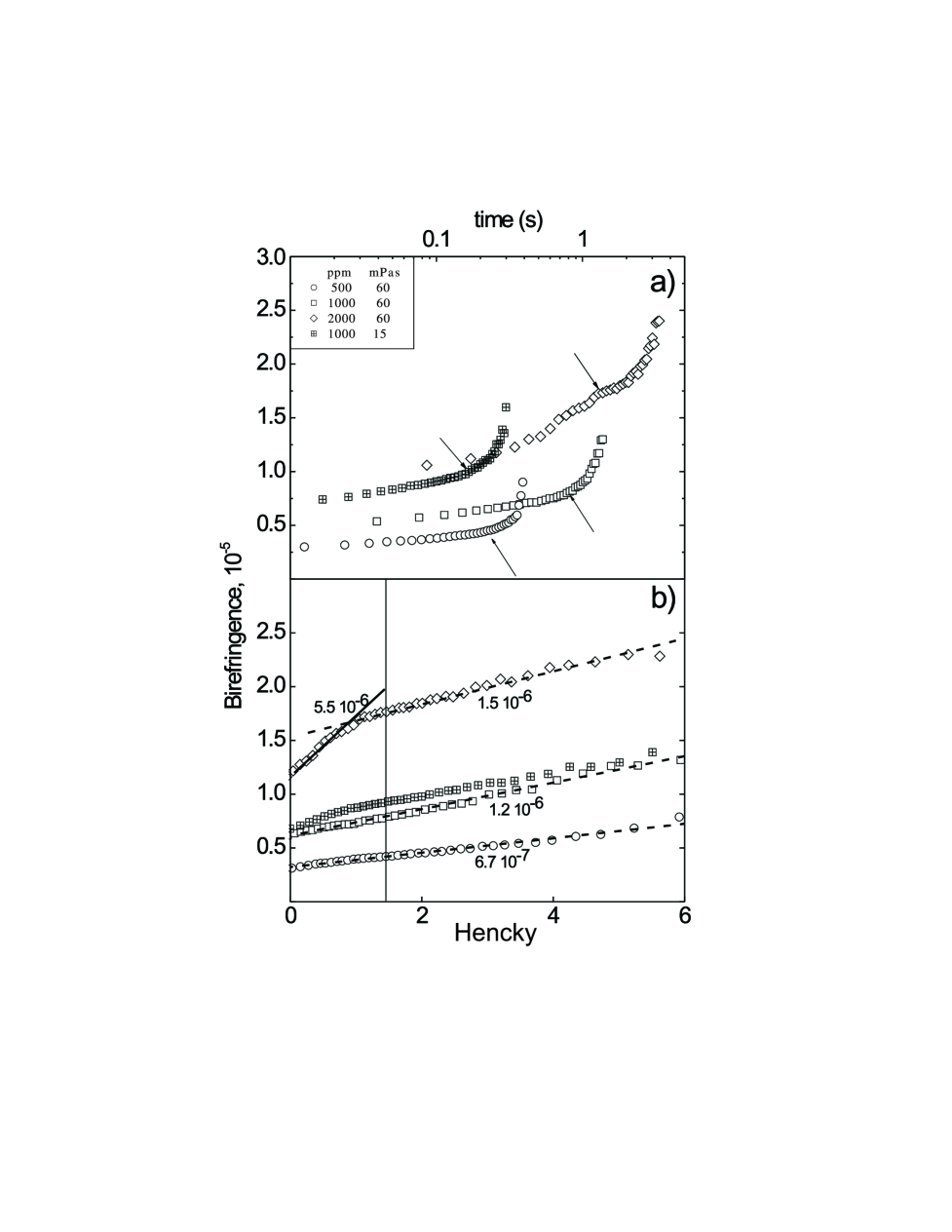
FIG. 7.: a) The instantaneous birefringence versus the elapsed time. The arrows indicate a Hencky strain of $\zeta=1.5$ b) the instantaneous birefringence versus the Hencky strain. The vertical line indicates the $\zeta=1.5$ position, the dashed lines are linear fits with slopes indicated by the numbers. Symbols are as in fig. 1.

However, instead of a plateau value at the final stage of the experiment, we observe a divergence in the birefringence signal (fig. 7a). The divergence is very reproducible and takes place at stages of the filament thinning process when the filament diameter is still large enough to render the analysis unambiguous. The divergence of the birefringence signal comes along with a divergence in the elongational rate $\dot{\epsilon}$ that follows from the linear shrinking of the filament. Surprisingly, we find that, the birefringence signal continues to increase with constant slope from $\zeta=1.5$ to $\zeta=6$ if plotted against the strain. Only for the $c_{p}\geq 1500ppm$ solutions did we observe a steeper slope in the birefringence signal for $\zeta<1.5$, presumably because of the stronger entanglement of the polymers.

While the polymers should be completely uncoiled in the linear thinning regime, additional physical mechanisms, that we will discuss in the following, have to be considered. We do see three different possible scenarios: first an effect of the polydispersity of the molecular weight distribution of our sample. But the observed large Wi should lead to a complete stretching of smaller molecules at even smaller strains. Second an overstretching of the molecule by the strong flow that would affect the configurations of the molecular bonds. Third a concentration enhancement by drainage or evaporation of the solvent. This picture is supported by the observation that, eventually, the filament might not break at the final stages of the thinning process but leave a very thin polymer ($<10\mu m$) fiber between the nozzle and the ground plate. Then a configuration called beads on a string occurs via an instability of the surface of the cylindrical filament [27].

V Conclusion

In conclusion, we have presented the first measurements on the molecular configurations of semi-rigid Xanthan molecules in a droplet detachment process of a complex liquid. We find that stiff molecules like Xanthan are highly oriented and stretched by the flow, even before the abrupt transition from the Newtonian self similar shrinking law to the exponential behavior of the elastic filament. Furthermore, we do observe a further increase of the birefringence signal after the saturation of elastic effects and the stretching of the polymers. We discussed different possible reasons for this phenomenon and find that a concentration enhancement is most likely to be the pertinent effect, but we cannot exclude the possibility that changes in the intramolecular bond configurations caused by the violent flow affect the birefringence signal too.

REFERENCES

- [1] For a review see: J. Eggers, Rev. Mod. Phys. 69, 865 (1997).
- [2] M. Goldin, J. Yerushalmi, R. Pfeffer, and R. Shinnar, J. Fluid. Mech. 38, 689 (1969).
- [3] A.V. Bazilevskii, V.M. Entov, and A.N. Rozhkov, Sov. Phys. Dokl. 26, 333 (1981).
- [4] Y. Amarouchene, D. Bonn, J. Meunier, and H. Kellay, Phys. Rev. Lett. 86, 3558 (2001).
- [5] L.B. Smolka, and A. Belmonte, J. Non Newt. Mech. 137, 103 (2006)
- [6] J. Li, and M.A. Fontelos, Phys. Fluids 15, 922 (2003).
- [7] G.G. Fuller, ”Optical rheometry of complex fluids”, Oxford University Press (1995).
- [8] G.H. Koenderink, S. Sacanna, D.G.A.L. Aarts, and A.P. Philipse, Phys. Rev. E 69, 021804 (2004) and references therein.
- [9] G. Holzwarth, and E.B. Prestridge, Science 197 758 (1977). W.E. Rochefort, and S. Middleman, J. Rheol. 31 337 (1987).
- [10] F.V. Lopez, L. Pauchard, M. Rosen, and, M. Rabaud J. Non Newt. Fluid Mech. 103, 123-139 (2002).
- [11] R.I. Tanner, ”Engineering Rheology”, OxfordScience (1985).
- [12] W. H. Talbot, and J.D. Goddard, Rheol. Acta 18 505(1979).
- [13] A. Rothert, R. Richter , and I. Rehberg, Phys. Rev. Lett. 87, 084501 (1901).
- [14] C.Wagner, Y.Amarouchene, Daniel Bonn, and J. Eggers, Phys. Rev. Lett. 95, 164504 (2005).
- [15] J.Eggers, Phys. Rev. Lett. 71, 3458 (1993).
- [16] V.M. Entov, and A.L. Yarin, Fluid. Dyn. 19, 21 (1984).
- [17] S.L. Anna, and G.H. McKinley, J. Rheol. 45, 115 (2000).
- [18] C. Wagner, P. Doyle, Y. Amarouchene, and D. Bonn Eur. Phys. Lett 64, 823 (2003).
- [19] Bird, Curtiss, Armstrongv and Hassager ”Dynamics of polymeric liquids”, J. Wiley (1987).
- [20] G.G. Fuller , C.A. Cathey , B. Hubbard, and B.E. Zebrowski, J. Rheol. 31, 235 (1987).
- [21] M. Khagram , R.K. Gupta and T. Sridhar J. Rheol. 29 191 (1985).
- [22] A. Mongruel, and B. Cloitre , J. Non Newt. Fluid Mech. 110, 27 (2002).
- [23] T.T. Perkins, D.E. Smith, and S. Chu, Science 276, 2016 (1997). D.E. Smith, and S. Chu, Science 281, 1335 (1998).
- [24] G. Maret, and G. Weill, Biopolymers 22, 2727 (1983).
- [25] N.P. Yevlamppieva, G.M., Pavlov and E.I. Rjumtsev, Int. J. Biol. Macromolecules 26, 295 (1999).
- [26] V.J. Morris, K. l Anson, and C. Turner, Int. J. Biol. Macromolecules 4, 362 (1982).
- [27] M.S.N. Oliveira and, G.H McKinley, Phys. Fluids ( 17, 071794 (2005).