Equilibrium statistical mechanics for single waves and wave spectra in Langmuir wave-particle interaction

Abstract

Under the conditions of weak Langmuir turbulence, a self-consistent wave-particle Hamiltonian models the effective nonlinear interaction of a spectrum of $M$ waves with $N$ resonant out-of-equilibrium tail electrons. In order to address its intrinsically nonlinear time-asymptotic behavior, a Monte Carlo code was built to estimate its equilibrium statistical mechanics in both the canonical and microcanonical ensembles. First the single wave model is considered in the cold beam/plasma instability and in the O’Neil setting for nonlinear Landau damping. O’Neil’s threshold, that separates nonzero time-asymptotic wave amplitude states from zero ones, is associated to a second order phase transition. These two studies provide both a testbed for the Monte Carlo canonical and microcanonical codes, with the comparison with exact canonical results, and an opportunity to propose quantitative results to longstanding issues in basic nonlinear plasma physics. Then the properly speaking weak turbulence framework is considered through the case of a large spectrum of waves. Focusing on the small coupling limit, as a benchmark for the statistical mechanics of weak Langmuir turbulence, it is shown that Monte Carlo microcanonical results fully agree with an exact microcanonical derivation. The wave spectrum is predicted to collapse towards small wavelengths together with the escape of initially resonant particles towards low bulk plasma thermal speeds. This study reveals the fundamental discrepancy between the long-time dynamics of single waves, that can support finite amplitude steady states, and of wave spectra, that cannot.

I Introduction

Wave-particle interaction is a universal phenomenon in space and laboratory plasmas. Its importance ranges from magnetic confinement fusion devices, in particular with its relation to anomalous transport or supplementary heating, to laser plasma interaction, astrophysics and charged particle beam physics. It is responsible for high-frequency plasma turbulence which differs substantially from low-frequency fluid or magnetohydrodynamic turbulence. In this article, we shall consider one of the simplest wave-particle interaction settings, namely electrostatic wave-particle interaction taking place in bump-on-tail or weak beam-plasma instabilities.

Under the conditions of weak Langmuir turbulence Sagdeev , electrostatic wave-particle interaction may be modeled Mynick78 ; CaryDoxas93 ; TMM ; AEE98 ; book by a reduced system coupling self-consistently a set of $M$ longitudinal (Langmuir) waves to $N$ quasi-resonant tail particles. This approach is especially appropriate to the description of basic plasma kinetic phenomena such as the bump-on-tail instability discrete or Landau damping phasetransition . In this reduced framework, the effective dynamics is ruled by a $(M+N)$-dimensional Hamiltonian system. More specifically, particles in the background plasma (whose velocities are roughly smaller than the thermal velocity) only participate to the dynamics via a small subset of collective modes, the Langmuir (long-wavelength) modes of longitudinal oscillation around their guiding-center positions. These modes are described by action-angle variables $\left(I_{j},\theta_{j}\right)$ with $1\leq j\leq M$ for the $M$ waves. In the absence of resonant particles, they oscillate with constant angular frequencies $d\theta_{j}/dt=\omega_{0j}$, that, according to the Bohm-Gross dispersion relation, are approximately equal to the plasma frequency $\omega_{p}$ for long-wavelength modes. These waves strongly interact with those plasma particles in the tails of the distribution function having velocities $v$ close to $\omega_{0j}/k_{j}$. The coupling is controlled by the small parameter $\eta$ that is the ratio of the tail density over the bulk plasma density. The dynamics of $N$ identical quasi-resonant particles moving on the interval of length $L$ with periodic boundary conditions, with unit mass and charge, and respectively position $x_{r}$ and momentum $p_{r}$, interacting with $M$ waves with wavenumbers $k_{j}=j2\pi/L$, derives then from the Hamiltonian

$$H^{N,M}=\sum\limits_{l=1}^{N}\frac{p_{l}^{2}}{2}+\sum_{j=1}^{M}\omega_{0j}I_{j}-\sqrt{\frac{2\eta}{N}}\sum\limits_{l=1}^{N}\sum_{j=1}^{M}\frac{\omega_{0j}^{3/2}\sqrt{I_{j}}}{k_{j}}\cos\left(k_{j}x_{l}-\theta_{j}\right).$$ (1)

Equations of motion are then

$$\dot{x}_{l} = p_{l},$$ (2)

$$\dot{p}_{l} = -\sqrt{\frac{2\eta}{N}}\sum_{j=1}^{M}\omega_{0j}^{3/2}\sqrt{I_{j}}\sin\left(k_{j}x_{l}-\theta_{j}\right),$$ (3)

$$\dot{\theta}_{j} = \omega_{0j}+\frac{\omega_{0j}^{3/2}}{2}\sqrt{\frac{2\eta}{NI_{j}}}\sum\limits_{l=1}^{N}\cos\left(k_{j}x_{l}-\theta_{j}\right),$$ (4)

$$\dot{I}_{j} = \sqrt{\frac{2\eta}{N}}\sum\limits_{l=1}^{N}\frac{\omega_{0j}^{3/2}\sqrt{I_{j}}}{k_{j}}\sin\left(k_{j}x_{l}-\theta_{j}\right).$$ (5)

It is important here to insist on the principle of this derivation: the background plasma is assumed to respond linearly to the waves which is valid provided resonant particles, whose velocities are much larger than plasma thermal velocity, only form a small fraction, $\eta$, of the total plasma. Moreover it is interesting to note that the same kind of wave-particle reduction has been undertaken for other physical regimes of wave-particle interaction. In particular, a Hamiltonian self-consistent wave-particle model KRAFFT05 has recently been built in order to study the nonlinear interaction of a packet of waves with a nonequilibrium electron distribution in a magnetized background plasma.

Under the above hypotheses, the Hamiltonian model (1) contains the effective dynamics of weak Langmuir turbulence. Yet, if a Hamiltonian system exhibits some ergodicity, then thermodynamics states that time averages can be replaced with equivalent space averages over the microcanonical ensemble. A Monte Carlo code was built to estimate the equilibrium statistical mechanics of (1) in both the canonical and microcanonical ensembles. This provides an efficient tool to investigate the time-asymptotic fate of the wave-particle model and discuss the evolution of weak Langmuir turbulence. This is of particular interest in the broad spectrum case where direct thermodynamical derivations are difficult.

In Section II, we present the canonical ensemble of the $M$ waves/$N$ particles self-consistent Hamiltonian model and focus on the $M=1$ case. In Sec. III, we consider the cold beam/plasma instability where the single wave approximation is particularly appropriate. Then, in Sec. IV, we apply the single wave model to the original O’Neil setting ONeil1965 for nonlinear Landau damping and, in parallel with microcanonical Monte Carlo results, associate O’Neil’s threshold to a second order phase transition. These two studies provide both a testbed for the Monte Carlo canonical and microcanonical codes, with the comparison with exact canonical results, and an opportunity to propose quantitative results to longstanding issues in basic nonlinear plasma physics. It is shown that statistical mechanics is a useful quantitative tool to address the nonlinear time-asymptotic saturation stage. Quantitative comparisons with experiments are given. Then, in Sec. V, we turn to the properly speaking weak turbulence framework by considering the case of a large spectrum of waves. We focus on the small coupling limit, as a benchmark for the statistical mechanics of weak Langmuir turbulence. We show that Monte Carlo microcanonical results fully agree with an exact microcanonical derivation. We conclude by discussing the predicted time-asymptotic spectrum, its relation to quasilinear theory and to a pending debate in theoretical, experimental and numerical plasma physics on the long time fate of the electric field for Landau damping.

II Canonical ensemble

We shall start deriving statistical mechanics in the canonical ensemble and then use the equivalence between canonical and microcanonical ensembles. Apart from the energy, it can be easily checked that the average total momentum per particle, $\sigma$, is also conserved with

$$\sigma=p+\frac{1}{N}\sum_{j=1}^{M}k_{j}I_{j},$$ (6)

and

$$p=\frac{1}{N}\sum_{l=1}^{N}p_{l}.$$ (7)

We introduce the new particle momenta $\bar{p}_{l}=p_{l}-p$ and the reduced wave intensities

$$\psi_{j}=\frac{I_{j}}{N},$$ (8)

that are properly normalized with respect to the $N\rightarrow\infty$ limit kinetic98 . Then, introducing (6), (1) reads

$$H=\sum\limits_{l=1}^{N}\frac{\bar{p}_{l}^{2}}{2}+\frac{N}{2}\left(\sigma-\sum_{j=1}^{M}k_{j}\psi_{j}\right)^{2}+N\sum_{j=1}^{M}\omega_{0j}\psi_{j}-\sum\limits_{l=1}^{N}\sum_{j=1}^{M}\sqrt{2\eta\psi_{j}}\omega_{0j}^{3/2}\cos\left(k_{j}x_{l}-\theta_{j}\right).$$ (9)

The canonical partition function is $Z_{c}(N,\beta)=Z_{0}(N,\beta)Z_{1}(N,\beta,\sigma)$, with

$$Z_{0}(N,\beta) = \int\prod\limits_{l=1}^{N}d\bar{p}_{l}\exp\left(-\beta\sum\limits_{l=1}^{N}\frac{\bar{p}_{l}^{2}}{2}\right)\delta\left(\sum_{l=1}^{N}\bar{p}_{l}\right)=\frac{1}{\sqrt{N}}\left(\frac{2\pi}{\beta}\right)^{(N-1)/2},$$ (10)

$$Z_{1}(N,M,\beta,\sigma) = N^{M}L^{N}\int\prod\limits_{j=1}^{M}d\psi_{j}d\theta_{j}\exp\left[-N\beta g(\beta,\sigma,\mathbf{\psi},\mathbf{\theta)}\right],$$ (11)

where

$$g(\beta,\sigma,\mathbf{\psi},\mathbf{\theta)=}\frac{1}{2}\left(\sigma-\sum_{j=1}^{M}k_{j}\psi_{j}\right)^{2}+\sum_{j=1}^{M}\omega_{0j}\psi_{j}-\beta^{-1}\ln\mathcal{I}(\beta,\mathbf{\psi},\mathbf{\theta}),$$ (12)

and

$$\mathcal{I}(\beta,\mathbf{\psi},\mathbf{\theta})=\frac{1}{L}\int_{0}^{L}dx\exp\left(\beta\sqrt{2\eta}\sum_{j=1}^{M}\frac{\omega_{0j}^{3/2}\sqrt{\psi_{j}}}{k_{j}}\cos\left(k_{j}x-\theta_{j}\right)\right).$$ (13)

All the difficulty lies in the estimation of (13) for $M>1$. We shall then first restrict our discussion to the case where only one mode is selected before going to the large-$M$ case in the small-coupling limit in Sec. V. The $M=1$ case occurs naturally in the cold beam-plasma interaction ONeil1965 ; ONeil71 ; TMM ; delCastillo2000 . We get, for $k=1$ and $L=2\pi$,

$$\mathcal{I}(\beta,\psi,\theta)=\frac{1}{2\pi}\int_{0}^{2\pi}dx\exp\left(\beta\omega_{0}^{3/2}\sqrt{2\eta\psi}\cos\left(x-\theta\right)\right)=I_{0}\left(\beta\omega_{0}^{3/2}\sqrt{2\eta\psi}\right).$$ (14)

This gives

$$g(\beta,\sigma,\psi,\theta)=\frac{1}{2}\left(\sigma-\psi\right)^{2}+\omega_{0}\psi-\beta^{-1}\ln\left[I_{0}\left(\beta\omega_{0}^{3/2}\sqrt{2\eta\psi}\right)\right].$$ (15)

Note here that in this particular case $g(\beta,\sigma,\psi,\theta)$ is actually independent of $\theta$. To perform the $\psi$ integral, we use Laplace’s method, for which we need to find the value $\psi^{\ast}$ of $\psi$ for which $g(\beta,\sigma,\psi,\theta)$ becomes a minimum. We get

$$\frac{\partial g}{\partial\psi}=\psi+\omega_{0}-\sigma-\frac{\eta\beta\omega_{0}^{3}}{\beta\omega_{0}^{3/2}\sqrt{2\eta\psi}}\frac{I_{1}\left(\beta\omega_{0}^{3/2}\sqrt{2\eta\psi}\right)}{I_{0}\left(\beta\omega_{0}^{3/2}\sqrt{2\eta\psi}\right)}=0$$ (16)

for

$$\psi^{\ast}=\sigma-\omega_{0}+\eta\beta\omega_{0}^{3}\frac{I_{1}\left(\beta\omega_{0}^{3/2}\sqrt{2\eta\psi^{\ast}}\right)}{\beta\omega_{0}^{3/2}\sqrt{2\eta\psi^{\ast}}I_{0}\left(\beta\omega_{0}^{3/2}\sqrt{2\eta\psi^{\ast}}\right)}.$$ (17)

We have, $\forall\psi\geq 0$, $\partial g/\partial\psi\geq\left.\partial g/\partial\psi\right|_{0}=\omega_{0}-\sigma-\eta\beta\omega_{0}^{3}/2$. If $\omega_{0}-\sigma-\eta\beta\omega_{0}^{3}/2\geq 0$, $g$ attains its minimum at the boundary, namely in $\psi=0$. Otherwise, there exists a unique minimum in $\psi^{\ast}>0$ satisfying (17). Transition occurs for the critical

$$\beta_{c}=\frac{2\left(\omega_{0}-\sigma\right)}{\eta\omega_{0}^{3}}.$$ (18)

We have then

$$Z_{1}(N,\beta,\sigma) = 2\pi N\int_{0}^{\infty}d\psi\exp\left[-N\beta g(\beta,\sigma,\psi\mathbf{)}\right]$$

$$\simeq 2\pi N\exp\left[-N\beta g(\beta,\sigma,\psi^{\ast}\mathbf{)}\right]\int_{0}^{\infty}d\psi\exp\left[-\frac{N\beta}{2}\left.\frac{\partial^{2}g}{\partial\psi^{2}}\right|_{\psi^{\ast}}(\psi-\psi^{\ast})^{2}\right]$$

$$= \pi N\exp\left[-N\beta g(\beta,\sigma,\psi^{\ast}\mathbf{)}\right]\sqrt{\frac{2\pi}{N\beta\left.\frac{\partial^{2}g}{\partial\psi^{2}}\right|_{\psi^{\ast}}}}\left[1+\mathop{\mathrm{erf}}\left(\sqrt{\frac{N\beta}{2}\left.\frac{\partial^{2}g}{\partial\psi^{2}}\right|_{\psi^{\ast}}}\psi^{\ast}\right)\right].$$

The ensemble average of the wave intensity is then simply

$$\left\langle I\right\rangle_{c}(N,\beta,\sigma)=N\psi^{\ast}\left(\beta,\sigma\right)+o(N),$$ (19)

meaning that the wave intensity is extensive when $\psi^{\ast}>0$, and non-extensive when $\psi^{\ast}=0$. The mean intensity $I/N$ acts as an order parameter (see Ref. phasetransition ): If $\beta_{c}<0$, then $\psi^{\ast}$ is always positive; yet, if $\beta_{c}>0$, then for $\beta<\beta_{c}$ (high temperature regime), $\psi^{\ast}=0$ meaning that, as $t\rightarrow\infty$, the wave intensity $\psi$ should vanish and particle motions should be ballistic, whereas for $\beta>\beta_{c}$ (low temperature regime), $\psi^{\ast}>0$ meaning that the wave intensity $\psi$ should be finite as $t\rightarrow\infty$.

III The single wave case: saturation of the cold beam/plasma interaction

III.1 Presentation

The analysis of O’Neil and Drummond et al. ONeil71 ; Drummond70 have shown that, in the case of a monokinetic beam, only a single wave, the wave having the largest growth rate, has a significant interaction with the beam, at least up to the first trapping oscillations. We shall consider here this single wave case and retain one mode ($M=1$) with rest frequency $\omega_{0}=\omega_{p}$ and wave number $k=1$. A simple linear analysis ONeil71 ; these determines then which initial beam streaming velocity $v_{b}$ leads to the maximal destabilization of this mode. This gives $v_{b}=\left(1+2^{-4/3}\eta^{1/3}\right)\omega_{p}$ and associated maximal linear growth rate $\gamma_{L}=2^{-4/3}\sqrt{3}\eta^{1/3}\omega_{p}$. This derivation is analogous to considering the more realistic scenario where the initial cold beam velocity is given and determining the dominant mode, namely the mode, among a continuum of modes, that is the most strongly destabilized. The expression of $v_{b}$ reveals the weakly resonant nature of the linear instability: it concerns mostly particles having velocities not equal to the initial wave velocity but about $\gamma_{L}/k$ away from it Zekri93 . Fig. 1 shows the time evolution of the wave intensity starting from an infinitesimal value. Nonlinear effects, namely trapping of particles in the wave trough, stop the initial linear exponential growth. Trapping oscillations coincide with the existence of a strong density inhomogeneity in the phase space. This is visible on the phase space snapshot in Fig. 2.

Figure 1: Wave intensity $\psi=I/N$ as a function of time (in $\omega_{p}^{-1}$ units) in the cold beam case for $N=10000$ and $\eta=3.85\times 10^{-5}$ (plain line). For the same parameters, ensemble averages of $\psi$ as a function of the number of Monte Carlo iterations for the microcanonical ensemble (bold line) and for the canonical ensemble with $U=E_{0}$ (dots) (See Sec. III.2).

Figure 2: Snapshot of the one-particle phase space in the wave frame for $t=5000\omega_{p}^{-1}$. Instantaneous separatrices of the wave resonance are shown. Dots represent the $N=10000$ particles, which were initially distributed uniformly in $x$ with the same velocity $v_{b}$.

III.2 Dynamical and Monte Carlo simulations; Canonical approach

We shall use the $M=1$ cold beam instability TMM as a simple testbed for the Monte Carlo code. Let us then first derive the canonical ensemble average of the wave intensity in this case and look for an analytical estimate as a function of the problem parameters and initial data.

The canonical ensemble average of energy is

$$U=-\partial_{\beta}\ln Z_{c}=-\partial_{\beta}\ln Z_{0}(N,\beta)-\partial_{\beta}\ln Z_{1}(N,\beta,\sigma),$$ (20)

with

$$-\partial_{\beta}\ln Z_{0}(N,\beta)=\frac{N-1}{2\beta},$$ (21)

and

$$-\partial_{\beta}\ln Z_{1}(N,\beta,\sigma)=Ng(\beta,\sigma,\psi^{\ast}\mathbf{)}+o(N).$$ (22)

This gives, with $\varepsilon\equiv U/N$,

$$\varepsilon=\frac{1}{2\beta}+\frac{1}{2}\left(\sigma-\psi^{\ast}\right)^{2}+\omega_{p}\psi^{\ast}-\beta^{-1}\ln\left[I_{0}\left(\beta\omega_{0}^{3/2}\sqrt{2\eta\psi^{\ast}}\right)\right],$$ (23)

that has to be solved together with (17). As given above, we have $\sigma-\omega_{p}=c\eta^{1/3}\omega_{p}$ with $c=2^{-4/3}$.

Let us look for solutions such that $\omega_{b\ast}^{2}\equiv\sqrt{2\eta\psi^{\ast}}\omega_{p}^{3/2}=a\eta^{\alpha}\omega_{p}^{2}$. Then (17) yields

$$\psi^{\ast}=c\eta^{1/3}\omega_{p}+\frac{I_{1}\left(\beta a\eta^{\alpha}\omega_{p}^{2}\right)}{aI_{0}\left(\beta a\eta^{\alpha}\omega_{p}^{2}\right)}\eta^{1-\alpha}\omega_{p}=\frac{a^{2}}{2}\eta^{2\alpha-1}\omega_{p}.$$ (24)

A maximal ordering in (24) is obtained for $\beta a\eta^{\alpha}\omega_{p}^{2}$ finite. It gives $1-\alpha=1/3=2\alpha-1$, that is $\alpha=2/3$. It is important to note that this corresponds to the trapping scaling for the wave intensity saturation, namely the asymptotic trapping frequency, $\omega_{b\ast}$, scales as the linear growth rate: $\omega_{b\ast}\sim\eta^{1/3}\omega_{p}\sim\gamma_{L}$. Introducing the finite quantity $d\equiv\beta a\eta^{2/3}\omega_{p}^{2}$, we have then

$$\frac{I_{1}\left(d\right)}{I_{0}\left(d\right)}=a\left(\frac{a^{2}}{2}-c\right)\equiv F_{1}(d),$$ (25)

and

$$\frac{\varepsilon}{\omega_{p}^{2}}=\frac{1}{2}+c\eta^{1/3}+\frac{a}{d}\left(\frac{1}{2}-\ln I_{0}\left(d\right)\right)\eta^{2/3}+\frac{1}{2}\left(\frac{a^{2}}{2}-c\right)^{2}\eta^{2/3}.$$ (26)

Let us now assume that the canonical average of the energy density, $\varepsilon$, is close to its initial value, $\varepsilon_{0}=E_{0}/N$. Because the wave intensity is initially vanishingly small, the identification $\varepsilon=\varepsilon_{0}$ gives for the cold beam case under consideration

$$\frac{\left\langle p^{2}\right\rangle_{0}}{2}=\frac{\sigma^{2}}{2}=\frac{\omega_{p}^{2}}{2}\left(1+c\eta^{1/3}\right)^{2}.$$ (27)

This gives finally

$$a\left(c-\frac{a^{2}}{4}\right)=\frac{1-2\ln I_{0}\left(d\right)}{d}\equiv F_{2}(d),$$ (28)

to be solved together with (25). We get

$$a=2^{2/3}\left[F_{1}(d)+F_{2}(d)\right]^{1/3}=c^{-1}\left(F_{1}(d)+2F_{2}(d)\right).$$ (29)

Using $c=2^{-4/3}$, this yields

$$\frac{\left[\frac{I_{1}\left(d\right)}{I_{0}\left(d\right)}+\left(\frac{1-2\ln I_{0}\left(d\right)}{d}\right)\right]^{1/3}}{\frac{I_{1}\left(d\right)}{I_{0}\left(d\right)}+2\left(\frac{1-2\ln I_{0}\left(d\right)}{d}\right)}=2^{2/3}.$$ (30)

This gives numerically $d\simeq 1.56$ and $a\simeq 1.313$, yielding, with (24) and in the limit $N\rightarrow\infty$,

$$\psi^{\ast}=\left\langle\frac{I}{N}\right\rangle_{c}\simeq 0.86\eta^{1/3}\omega_{p}+o(1).$$ (31)

Dynamical symplectic CaryDoxas93 simulations indicate that, after some trapping periods, the average wave intensity $I/N$ scales approximately as $0.78\eta^{1/3}$ these . For the parameter $\eta$ chosen in Fig. 1, this gives $\left\langle I/N\right\rangle_{\mu}\simeq 0.026$ as $N\rightarrow\infty$ which is indeed in agreement with the time average of $\psi$. The microcanonical Monte Carlo results plotted on the same Figure show an excellent agreement with this time average. Canonical Monte Carlo results assuming $U=N\varepsilon_{0}$ is in fine agreement with the analytical result (31). This is a practical way to bypass the microcanonical or time-asymptotic evaluation of $\beta$ and relate directly canonical results to initial data. Here this result shows a ten-per-cent discrepancy with the exact microcanonical result. Moreover, we can equivalently express Eq. (31) in terms of the ratio between the asymptotic trapping pulsation and the linear growth rate yielding

$$\frac{\omega_{b\ast}}{\gamma_{L}}=\frac{\left(2\eta\psi^{\ast}\right)^{1/4}\omega_{p}^{3/4}}{2^{-4/3}\sqrt{3}\eta^{1/3}\omega_{p}}\simeq\frac{\left(2\times 0.86\right)^{1/4}}{2^{-4/3}\sqrt{3}}=1.67.$$ (32)

This is in agreement with the results of an early experiment by Mizuno and Tanaka Mizuno72 designed to test the single wave model. A monoenergetic beam is injected along a homogeneous magnetic field, making the system unidimensional, into a plasma. In this electron gun, the mechanism of the nonlinear saturation of a nearly single wave is reported through the first measurement of the trapping of beam electrons. The approximate experimental value, given in Ref. Mizuno72 , of the ratio $\omega_{b}/\gamma_{L}$ associated to the first trapping pulsation is 0.83. As evidenced by Fig. 1, this can here be used as a fairly good approximation of the asymptotic value $\omega_{b\ast}/\gamma_{L}$. Yet, proceeding to a direct measure from the data plotted on the Figure 1 of Ref. Mizuno72 , we obtain a somewhat larger value for this quantity, slightly above 1.2 and closer to the estimate (32).

Finally, it is interesting to note that an explicit low-dimensional modeling of the dynamics, along the lines of Ref. TMM stressing the phase space division between the macroparticle and chaotic sea components, has been recently proposed by Antoniazzi et al. in the saturated regime of a single pass free electron laser around perfect tuning AEFR2006 . This model uses an Hamiltonian formulation that is a direct counterpart of the present Hamiltonian single-wave particle framework.

IV Landau damping of a single wave: Phase transition and O’Neil’s threshold

In Ref. ONeil1965 , O’Neil considered the damping of a single wave interacting effectively with a subset of resonant particles. He proposed a qualitative dynamical threshold conditioning the time asymptotic behavior of the wave: if the linear damping time $\left|\gamma_{L}\right|^{-1}$ is far smaller than the initial nonlinear trapping time $\tau_{b0}$ of the particles in the wave trough, then the wave should not have enough time to experience nonlinear effects and should be completely damped as $t\rightarrow\infty$. On the contrary, if the nonlinear time $\tau_{b0}$ is smaller than $\left|\gamma_{L}\right|^{-1}$, the linear one, nonlinear effects (trapping) should forever control the dynamics. This can be already inferred from a linear analysis. As already apparent in the cold beam case, the particles controlling the linear regime are those quasi-resonant particles located at about $\gamma_{L}/k$ from $\omega_{p}/k$ Zekri93 : if those particles are trapped in the initial wave (with half resonance width $2\omega_{b0}$) right away, then the linear regime should be bypassed. However, this result is qualitative. Actually, in spite of major recent advances in the analytical and computational fields Brodin97 ; Isi97 ; Manfredi97 ; LancellottiDorning ; Brunetti2000 ; Valentini05 ; DeMarco2006 ; Ivanov06 , mostly in the full Vlasov-Poisson framework, as well as in experiments Danielson04 , no definite answer presently exists to this intrinsically nonlinear and time-asymptotic issue, in the sense that no quantitative threshold separating nonzero time-asymptotic wave amplitude states from zero ones is known. This is basically due to the facts that analytical reductions of the problem should e.g. make some restrictions on the asymptotic behavior of the electric field whereas numerical and experimental investigations should be obviously taken with great care when addressing the $t\rightarrow\infty$ limit. For instance, the nice experiments recently done in a trapped pure electron plasma Danielson04 diagnose the first trapping oscillation frequency $\omega_{b}$ at the onset of the nonlinear stage (and more precisely the dimensionless ratio $\gamma_{L}/\omega_{b}$) as a function of the initial ratio $\gamma_{L}/\omega_{b0}$ rather than the, rigorously speaking, time-asymptotic state.

We shall consider here the single wave-particle interaction model that describes the effective (field envelope) dynamics of the Vlasov-Poisson system in the case where only one wave exists. This is obviously an idealized or academic situation, yet it is perfectly appropriate to discuss O’Neil’s picture. We shall show here that O’Neil’s threshold can be related to a second order phase transition for the single wave self-consistent Hamiltonian model $H^{N,1}$, with order parameter the wave intensity $\psi$. This was already discussed in Ref. phasetransition . We shall however consider here specifically the O’Neil setting, that is we take a given finite initial wave intensity $\psi_{0}$ and a monotonously decreasing, linear, tail particle distribution function $f_{0}(v)$, of which we shall vary the slope and thus the linear Landau damping rate $\gamma_{L}$ (See Fig. 3). Because of locality properties in the velocity space FirpoDoveil , the wave has an effective interaction only with particles that are not too far away from its separatrices. One can reasonably think that particles having velocities more than, let’s say, $4\omega_{b0}/k$ away from $\omega_{p}/k$ FirpoDoveil should evolve on Kolmogorov-Arnold-Moser (KAM) tori for the pendulum-like 1,5 degrees of freedom Hamiltonian (given by Eqs. (2)-(3) with $(I(t),\theta(t))$) associated to $H^{N,1}$, materializing the separation between the wave-particle interaction zone and the plasma bulk captured into the collective variable $I$.

Figure 3: Family of tail distribution functions. We shall take $\Delta=4\omega_{b0}/k$.

Let us then put $\omega_{p}=1$, define $\Delta=4\omega_{b0}=4\left(2\eta\psi_{0}\right)^{1/4}$ and take $f_{0}(v)=av+b$ if $v\in\left[1-\Delta;1+\Delta\right]$ and $f_{0}(v)=0$ otherwise, with $a<0$. Normalization imposes $b=(1-2a\Delta)/(2\Delta)$ and positivity $-a<(2\Delta^{2})^{-1}$. We have $\left\langle v\right\rangle_{0}=2a\Delta^{3}/3+1$  and $T_{0}\equiv\left\langle v^{2}\right\rangle_{0}-\left\langle v\right\rangle_{0}^{2}=-\Delta^{2}\left(4a^{2}\Delta^{4}-3\right)/9$. Let us now write the condition $\beta<\beta_{c}$ for which particle asymptotic behavior should be ballistic. From (23), we have in this regime

$$\left.\varepsilon\right|_{\psi^{\ast}=0}=\frac{1}{2\beta}+\frac{\sigma^{2}}{2}.$$ (33)

If we identify, once again, this canonical ensemble average with the initial density of energy in the system $\varepsilon_{0}=$ $\left\langle v^{2}\right\rangle_{0}/2+\psi_{0}$ and use $\sigma=\left\langle v\right\rangle_{0}+$ $\psi_{0}$, we get the following condition on the slope of the initial tail distribution:

$$\beta<\beta_{c}\Leftrightarrow Q(a)>\frac{27}{16}\eta\Delta^{-9}$$ (34)

where $Q$ is the third degree polynomial

$$Q(x) = \left(x-c_{+}\right)\left(x-c_{-}\right)\left(x-c\right)$$ (35)

$$\text{with \ }c_{\pm} \equiv c\pm\sqrt{3}/(2\Delta^{2}),c\equiv-3\Delta/(4^{5}\eta).$$ (36)

Moreover, to ensure $\beta_{c}>0$, one should have $\sigma<\omega_{0}$ i.e. $\left\langle v\right\rangle_{0}+\psi_{0}<1$ so that

$$a<c=-3\Delta/(4^{5}\eta).$$ (37)

$Q^{\prime}(x)$ vanishes for $d_{\pm}=c\pm 1/(2\Delta^{2})$, the relative maximum of $Q$ being reached in $d_{-}$. Taking into account the positivity condition $-a<(2\Delta^{2})^{-1}$, Eq. (37) and $d_{-}<-(2\Delta^{2})^{-1}$, one concludes that, in order to observe a phase transition for this family of initial tail distribution functions, it is necessary and sufficient that $Q(-(2\Delta^{2})^{-1})>27\eta\Delta^{-9}/16$. The necessary condition $Q\left(d_{-}\right)>\frac{27}{16}\eta\Delta^{-9}$ is easier to formulate and reads

$$\Delta>3\times 2^{-2/3}\eta^{1/3}\text{.}$$ (38)

The righthand side of (38) is reminiscent of the scaling law of the growth rate of the cold beam. This inequality is both a condition on the beam width and initial wave amplitude. In order to observe a regime in which the wave and the particles are decoupled in the sense that $I$ is no longer extensive (ballistic regime instead of trapping regime), it is necessary to exclude the case of a cold beam. In this latter case, even if the initial wave amplitude is infinitesimal, it will not be completely damped: this signals the singular character of the cold beam/wave interaction. Eq. (38) means that a wave interacting resonantly with a cold beam cannot be Landau damped to zero. Additionally, the condition (38) thus specifies what is meant by an ”initially finite” wave amplitude. The wave-particle interaction model à la O’Neil presented here rules out the classical research case of Landau damping in the limit of a perturbative wave of infinitesimal amplitude. The present framework is definitely non trivial since, if the wave is effectively damped asymptotically to zero, nonlinear effects should place the study in the frame of Isichenko’s resolution Isi97 predicting a very slow, asymptotically algebraic, damping.

Let us illustrate these results for values of $\Delta$ and $\eta$ allowing a phase transition in the canonical approach just described.

Figure 4: Monte Carlo microcanonical ensemble averages of the wave intensity $\psi=I/N$ as a function of the slope $a$ of the initial distribution function and corresponding $q$. For $N=10000$ particles, the microcanonical ensemble averages of the fluctuations $<(\psi-<\psi>_{\mu})^{2}>_{\mu}^{1/2}$ are indicated as errorbars.

Figure 5: Same as Fig. 4 in lin-log scale.

Taking $\Delta=0.25$ and $\eta=0.001$ gives $Q(-(2\Delta^{2})^{-1})=1011.5>\frac{27}{16}\eta\Delta^{-9}=442.37$, which ensures the existence of a phase transition. The tail distribution slope $a$ can vary between $-8$ and $0$, and the critical slope associated with (34) is $a_{c}=-3.106$. This corresponds to a linear Landau damping rate $\gamma_{Lc}=\left(\pi a_{c}\eta\right)/2=-4.88\times 10^{-3}$. We are now able to estimate the O’Neil threshold, namely the critical threshold of $q\equiv\left|\gamma_{L}\right|/\omega_{b0}$, as

$$q_{c}=\frac{\left|\gamma_{Lc}\right|}{\omega_{b0}}\simeq 0.078.$$ (39)

We can check that this value is very close to the threshold estimated in Ref. phasetransition in which the initial tail distribution (close to, but not, linear), and thus the linear Landau damping rate, was given whereas the initial wave amplitude was the control parameter. This agreement may be interpreted as an indicator of the robustness of the statistical mechanics approach. Figs. 4 and 5 show the Monte Carlo microcanonical ensemble averages of the wave intensity as a function of the slope of the initial tail distribution function and of the parameter $q$. A nice agreement with the threshold (39) is found. The transition is emphasized by the logarithmic scale in Fig. 5, as in the asymptotic ballistic regime, $\psi$ scales as $1/N$.

Using equilibrium statistical mechanics allows then to set in a quantitative way O’Neil’s threshold. However strong metastability effects and long relaxation times towards equilibrium in the vicinity of the phase transition phasetransition temper the practical interest of this result, especially in the purely collisionless Vlasovian $N\rightarrow\infty$ limit kinetic98 for which there is increasing evidence discrete ; Bouchet2005 ; Yoon that it may not commute with the $t\rightarrow\infty$ limit. This explains that practical experimental and numerical attempts to determine $q_{c}$ typically yield values that are about one order larger than (39). It should be also remembered that, as demonstrated by Isichenko’s calculation Isi97 , the asymptotic behavior of a damping electric field is intrinsically very slow, so very difficult to detect and discriminate practically from a Bernstein-Greene-Kruskal (BGK) saturation stage BGK . Equilibrium statistical mechanics should prove however essential to address the large time nonlinear fate of wave-particle interaction in the generic case of many waves. Strong resonances overlap may then create large scale chaos inducing an efficient sweeping of the phase space ensuring good ergodic properties or, using the Lynden-Bell terminology, violent relaxation.

V Microcanonical predictions for a large number of waves: the infinitesimal coupling limit

V.1 Motivations and Monte Carlo simulations

We shall consider here a regime for which the validity of quasilinear theory has been questioned ALP79 ; DoxasCary97 ; Laval99 , when the nonlinear timescale (resonance broadening time $\tau_{\mathrm{RB}}$) is much lower than the linear one (of the order of the inverse of the linear growth rate $\gamma_{L}$), that is $\mu\equiv(\tau_{\mathrm{RB}}\gamma_{L})^{-1}\gg 1$. Equilibrium predictions are expected to be particularly relevant for this problem since chaotic mixing and system ergodization should prove effective typically on the nonlinear timescale.

Let us begin by presenting microcanonical Monte Carlo simulations done for parameters very close to those used by Doxas and Cary in Ref. DoxasCary97 . Specifically, the wave spectrum is composed of $M=584$ waves, that are initially strongly overlapping with a Chirikov overlap parameter of about 500, with wavenumbers between 2.78 and 3.70. The strong overlap is needed to model a continuous spectrum. The beam distribution in velocity is the same as in Ref. DoxasCary97 , chosen to give a constant linear growth rate across the spectrum: $f_{0}(v)=C_{1}+C_{2}\left(1-v_{a}/v\right)$ if $v\in\left[v_{a};v_{b}\right]$ and $f_{0}(v)=0$ otherwise, with $C_{1}$ and $C_{2}$ fixed by normalization and the value of the growth rate. For the Monte Carlo code, these particular initial conditions just fix the two microcanonical constants of motion, namely the total energy and momentum. Then, as detailed in the analysis of Ref. DoxasCary97 , the large-$\mu$ regime is entered as the coupling (control) parameter $\eta$ becomes vanishingly small. We are thus investigating here the small coupling regime.

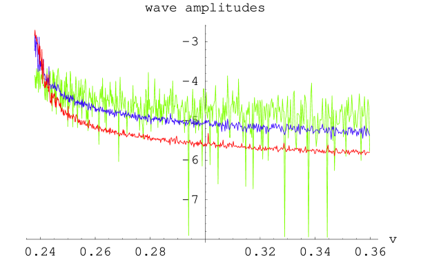
Figure 6: (Color Online) Wave spectrum obtained through microcanonical Monte Carlo simulations, for $\eta=2.6\times 10^{-4}$ and initial conditions described in the text, for two values of the number $N$ of particles: with $N=5000$ in the transient regime (after only a few iterations) (upper curve), with $N=5000$ at equilibrium (middle curve) and for $N=20000$ at equilibrium (lower curve). Wave amplitudes are given in logarithmic scale.

Results may be summarized as follows: in the transient stage of the Monte Carlo runs, that may be compared with some care to the real time dynamics, one observes ”noisy” wave spectra that may be related to the spontaneous spectra discretization reported in previous studies DoxasCary97 . In the thermodynamical framework, this appears only as a transient stage towards equilibration. The major point depicted by Fig. 6 is that the energy apparently tends to concentrate at equilibrium into a very small number of small wavelength modes while the long wavelength wave intensities are no longer extensive.

V.2 Exact microcanonical derivation

Let us consider analytically the small coupling limit, namely $\eta\rightarrow 0^{+}$. This is a singular limit that amounts to neglect (at zero order in $\eta$) the wave-particle interaction potential in the self-consistent Hamiltonian (1) while retaining the total wave-particle momentum conservation constraint. In the microcanonical ensemble, the partition function reads, with $\omega_{0j}=\omega_{p}$ for any wave number $j$,

$$Z_{\mu}(E,P)=\int\delta\left(E-\sum\limits_{l=1}^{N}\frac{p_{l}^{2}}{2}-\omega_{p}\sum_{j=1}^{M}I_{j}\right)\delta\left(P-\sum\limits_{l=1}^{N}p_{l}-\sum_{j=1}^{M}k_{j}I_{j}\right)d^{N}\mathbf{p}d^{M}\mathbf{I.}$$ (40)

Let us introduce $I_{j}^{\prime}=I_{j}$ for $1\leq j\leq M-1$ and $I_{M}^{\prime}$ such that $\sum_{j=1}^{M}I_{j}=\sum_{j=1}^{M-1}I_{j}^{\prime}+I_{M}=MI_{M}^{\prime}$. We get

$$Z_{\mu}(E,P)=M\int\delta\left(E-\sum\limits_{l=1}^{N}\frac{p_{l}^{2}}{2}-\omega_{p}MI_{M}^{\prime}\right)\delta\left(P-\sum\limits_{l=1}^{N}p_{l}-\sum_{j=1}^{M-1}\left(k_{j}-k_{M}\right)I_{j}^{\prime}-k_{M}MI_{M}^{\prime}\right)d^{N}\mathbf{p}d^{M}\mathbf{I}^{\prime}\mathbf{.}$$ (41)

Introducing

$$B\equiv\frac{k_{M}}{\omega_{p}}E+\frac{N\omega_{p}}{2k_{M}}-P,$$ (42)

integration over $I_{M}^{\prime}$ gives

$$Z_{\mu}(E,P) = M\int\delta\left(P-\sum\limits_{l=1}^{N}p_{l}-\sum_{j=1}^{M-1}\left(k_{j}-k_{M}\right)I_{j}^{\prime}-\frac{k_{M}}{\omega_{p}}E+\frac{k_{M}}{\omega_{p}}\sum\limits_{l=1}^{N}\frac{p_{l}^{2}}{2}\right)d^{N}\mathbf{p}\prod\limits_{j=1}^{M-1}dI_{j}^{\prime}$$ (43)

$$= M\int\delta\left(\sum_{j=1}^{M-1}\left(k_{M}-k_{j}\right)I_{j}^{\prime}-B+\sum\limits_{l=1}^{N}\left(\sqrt{\frac{k_{M}}{2\omega_{p}}}p_{l}-\sqrt{\frac{\omega_{p}}{2k_{M}}}\right)^{2}\right)d^{N}\mathbf{p}d^{M-1}\mathbf{I}^{\prime}$$

$$= M\left(\frac{2\omega_{p}}{k_{M}}\right)^{N/2}\int\delta\left(\sum_{j=1}^{M-1}\left(k_{M}-k_{j}\right)I_{j}^{\prime}-B+\sum\limits_{l=1}^{N}\tilde{p}_{l}^{2}\right)d^{N}\mathbf{\tilde{p}}d^{M-1}\mathbf{I}^{\prime}$$

It is requested that

$$0\leq\sum_{j=1}^{M-1}\left(k_{M}-k_{j}\right)I_{j}^{\prime}\leq B,$$ (44)

so that, in particular, with $\omega_{p}/k_{M}=v_{\theta\min}$,

$$v_{\theta\min}\sigma-\frac{v_{\theta\min}^{2}}{2}\leq\varepsilon.$$ (45)

This inequality (45) is basically satisfied when the particle impulsions are larger than the smallest wave velocity, which is the natural setting of the wave-particle interaction model. Eq. (43) is easily integrated over the $\tilde{p}_{l}$’s yielding, assuming $N$ even,

$$Z_{\mu}(E,P)=\frac{2M}{\pi\left(N/2-1\right)!}\left(\frac{2\pi\omega_{p}}{k_{M}}\right)^{N/2}\int f\left(\sum_{j=1}^{M-1}\left(k_{M}-k_{j}\right)I_{j}^{\prime}\right)d^{M-1}\mathbf{I}^{\prime},$$ (46)

with $f(x)\equiv\left(B-x\right)^{(N-1)/2}$ and where the integration boundaries are given $0\leq\sum_{j=1}^{M-1}\left(k_{M}-k_{j}\right)I_{j}^{\prime}\leq B$ with $0\leq I_{j}^{\prime}$, $\forall j$, $1\leq j\leq M-1$. We begin by making a change a variable, putting $\left(k_{M}-k_{j}\right)I_{j}^{\prime}=\tilde{I}_{j}$. This gives

$$Z_{\mu}(E,P)=\frac{2M}{\pi\left(N/2-1\right)!}\left(\frac{2\pi\omega_{p}}{k_{M}}\right)^{N/2}\prod\limits_{j=1}^{M-1}\left(k_{M}-k_{j}\right)^{-1}\int_{0\leq\sum_{j=1}^{M-1}\tilde{I}_{j}\leq B}f\left(\sum_{j=1}^{M-1}\tilde{I}_{j}\right)d^{M-1}\mathbf{\tilde{I}.}$$ (47)

We have

$$\int_{0\leq\sum_{j=1}^{M-1}\tilde{I}_{j}\leq B}f\left(\sum_{j=1}^{M-1}\tilde{I}_{j}\right)d^{M-1}\mathbf{\tilde{I}}$$

$$= \int d\tilde{I}_{M-1}\int\ldots\int\limits_{0}^{B-\sum_{j=2}^{M-1}\tilde{I}_{j}}d\tilde{I}_{1}\left(B-\sum_{j=1}^{M-1}\tilde{I}_{j}\right)^{(N-1)/2}$$

$$= \frac{1}{(N-1)/2+1}\int d\tilde{I}_{M-1}\int\ldots\int\limits_{0}^{B-\sum_{j=3}^{M-1}\tilde{I}_{j}}d\tilde{I}_{2}\left(B-\sum_{j=2}^{M-1}\tilde{I}_{j}\right)^{(N-1)/2+1}$$

$$= \prod_{j=1}^{M-2}\frac{1}{(N-1)/2+j}\int_{0}^{B}d\tilde{I}_{M-1}\left(B-\tilde{I}_{M-1}\right)^{(N-1)/2+M-2}$$

$$= \prod_{j=1}^{M-1}\frac{1}{(N-1)/2+j}B^{(N-1)/2+M-1}.$$

Finally, we get

$$Z_{\mu}(E,P)=\frac{2M}{\pi\left(N/2-1\right)!}\left(\frac{2\pi\omega_{p}}{k_{M}}\right)^{N/2}\times\prod_{j=1}^{M-1}\frac{\left(k_{M}-k_{j}\right)^{-1}}{(N-1)/2+j}\times\left[\frac{k_{M}}{\omega_{p}}E+\frac{N\omega_{p}}{2k_{M}}-P\right]^{(N-1)/2+M-1}.$$ (48)

Following the calculations presented in the Appendix A, we derive the wave intensities for any $j_{0}$ strictly smaller than $M$ as

$$\left\langle\psi_{j_{0}}\right\rangle_{\mu}^{(N)}\sim_{N\gg 1}\frac{1}{N}\frac{T_{\mu}}{\omega_{p}}\frac{v_{\theta j_{0}}}{v_{\theta j_{0}}-v_{\theta\min}}.$$ (49)

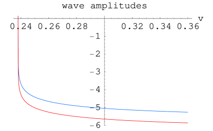
Figure 7: (Color Online) Equilibrium wave spectrum as derived in Eq. (49) for the same initial wave and particle distributions as in Fig. 6, for two values of the number $N$ of particles: for $N=5000$ (upper curve) and for $N=20000$ (lower curve). Wave amplitudes are given in logarithmic scale. Numerical data for the initial conditions are $v_{\theta\min}=0.2379$, $\varepsilon=0.0555$ and $\sigma=0.333$.

As shown on Fig. 7, this result nicely agrees with Monte Carlo microcanonical expectations in the limit $\eta\rightarrow 0^{+}$. We have introduced the microcanonical temperature $T_{\mu}$ through

$$\frac{1}{T_{\mu}}=\frac{\partial\ln Z_{\mu}}{\partial E}\sim\frac{1}{2}\frac{\frac{k_{M}}{\omega_{p}}}{\frac{k_{M}}{\omega_{p}}\varepsilon+\frac{\omega_{p}}{2k_{M}}-\sigma},$$ (50)

so that

$$\frac{T_{\mu}}{2}\sim\varepsilon+\frac{v_{\theta\min}^{2}}{2}-\sigma v_{\theta\min}.$$ (51)

This clarifies the inequality (45), that just means that the temperature $T_{\mu}$ should be positive. Let us now complete this study by moving to a grand canonical ensemble, that is both canonical with respect to the energy and the total momentum.

V.3 Grand canonical approach

We define

$$Z_{G}\left(\beta,\lambda\right)\equiv\int\exp\left(-\beta H-\lambda P\right)d^{N}\mathbf{p}d^{M}\mathbf{I,}$$ (52)

with $H=\sum_{l=1}^{N}\frac{p_{l}^{2}}{2}+\omega_{p}\sum_{j=1}^{M}I_{j}$ and $P=\sum_{l=1}^{N}p_{l}+\sum_{j=1}^{M}k_{j}I_{j}$. This gives immediately

$$Z_{G}\left(\beta,\lambda\right)=\left(\frac{2\pi}{\beta}\right)^{N/2}\exp\left(\frac{N\lambda^{2}}{2\beta}\right)\prod_{j=1}^{M}\left(\beta\omega_{p}+\lambda k_{j}\right)^{-1}.$$ (53)

In this ensemble, we easily derive

$$\left\langle I_{j_{0}}\right\rangle_{G}=\frac{1/\beta}{\left(\omega_{p}+k_{j_{0}}\lambda/\beta\right)}=\frac{v_{\theta j_{0}}/\beta}{\omega_{p}\left(v_{\theta j_{0}}+\lambda/\beta\right)},$$ (54)

with (see Appendix B)

$$\frac{\lambda}{\beta}=-\left\langle\frac{1}{N}\sum_{l=1}^{N}p_{l}\right\rangle_{G},$$ (55)

and the ensemble average of the reduced kinetic energy is found to be

$$\left\langle K\right\rangle_{G} \equiv \left\langle\sum_{l=1}^{N}\frac{1}{2}\left(p_{l}-\frac{1}{N}\sum_{k=1}^{N}p_{k}\right)^{2}\right\rangle_{G}$$

$$= \left\langle\sum_{l=1}^{N}\frac{p_{l}^{2}}{2}\right\rangle_{G}-\frac{1}{2N}\left\langle\left(\sum_{l=1}^{N}p_{l}\right)^{2}\right\rangle_{G}\sim\frac{N}{\beta}.$$

V.4 Discussion and conclusion

Considering a spectrum of waves, we have focused on the small coupling limit as a benchmark for the statistical mechanics of weak Langmuir turbulence. A trivial correspondence, assuming the equivalence of ensembles, between Eqs. (49) and (54), using (55), shows that electrons should, as time proceeds, escape from the original resonances towards lower speeds. Meanwhile, the wave spectrum collapses towards short-wavelengths and the wave energy eventually concentrates into the mode of minimal phase velocity, that basically matches plasma thermal velocity. Consistently, particles (electrons) behaving almost freely loose their resonant character and follow the decay of waves towards small velocities.

Let us then briefly comment on the relation of these results with the investigation on the limits of quasilinear theory undertaken by Doxas and Cary DoxasCary97 . It is obviously uneasy to draw conclusions on the out-of-equilibrium behavior, such as diffusion, from equilibrium statistical mechanics results. Some statements are still possible: When the nonlinear timescale is far larger than the linear one, quasilinear theory is expected not to apply as the timescale of validity of (almost) zero-order effects, such as the reaction of the resonant wave spectrum on the zero-order distribution function, becomes negligible. Actually, we infer from the equilibrium microcanonical results that, within some nonlinear thermalization timescale, the initial particle distribution function is substantially modified whereas the wave spectrum collapses towards the short wavelengths. The thermalization stage is expected to exhibit a noisy wave spectrum, as in Monte Carlo transients, as the wave spectrum collapse proceeds through higher order wave-wave couplings, which may explain the dynamical findings of diffusion enhancements DoxasCary97 .

Now, we can consider the small coupling results from a more general perspective. Let us consider an initial very weak beam-plasma or bump-on-tail instability destabilizing some spectrum of waves towards suprathermal levels in a wave-particle interaction dynamics captured by the self-consistent Hamiltonian (1). Then, the previous calculation predicts that this out-of-equilibrium dynamics cannot sustain itself as the wave energy should drop and cascade towards short-wavelengths with phase velocities reaching the plasma bulk thermal velocity. Obviously, the self-consistent Hamiltonian model reaches at this point its validity limit. This behavior is an effect of considering a spectrum of modes rather than single modes, as in Secs. III and IV, for which trapping ensures the long-standing stabilization of the instability.

Recently a pending debate emerged concerning the time-asymptotic state of a large amplitude Landau damped wave Danielson04 . It is commonly expected that the system will eventually enter some stationary BGK equilibrium with a time-asymptotic finite wave amplitude provided the initial amplitude is large enough. This agrees with the statistical mechanics predictions for a single wave derived in Sec. IV under the O’Neil setting. The existence of BGK steady states is supported by some theoretical analysis and numerical results Manfredi97 ; LancellottiDorning ; Brunetti2000 . However, Brodin’s numerical simulations Brodin97 suggested that the wave amplitude never settles to a steady value as the energy of the resonant particles diffuses slowly into higher harmonics. Moreover Isichenko Isi97 argued that nonlinearities should not stop the damping of the electric field towards a vanishing time-asymptotic amplitude. Our point of view here is that, within the weak coupling hypothesis - that besides fully justifies the linear response of the background plasma -, the Landau damping of a spectrum of waves is predicted not to reach a BGK finite amplitude steady state with the resonant tail electrons drifting with wave energy towards plasma bulk.

Appendix A Exact microcanonical ensemble averages of the wave intensities in the limit $\eta\rightarrow 0^{+}$

We wish to calculate

$$\left[I_{j_{0}}^{\prime}\right]^{(N)}\equiv\frac{2M}{\pi\left(N/2-1\right)!}\left(\frac{2\pi\omega_{p}}{k_{M}}\right)^{N/2}\int I_{j_{0}}^{\prime}\left(B-\sum_{j=1}^{M-1}\left(k_{M}-k_{j}\right)I_{j}^{\prime}\right)^{(N-1)/2}d^{M-1}\mathbf{I}^{\prime}.$$ (56)

We have

$$\frac{\partial Z_{\mu}^{(N+2)}}{\partial k_{j_{0}}}=\frac{2M}{\pi\left(N/2+1\right)!}\left(\frac{2\pi\omega_{p}}{k_{M}}\right)^{N/2+1}\frac{N+1}{2}\int I_{j_{0}}^{\prime}\left(B-\sum_{j=1}^{M-1}\left(k_{M}-k_{j}\right)I_{j}^{\prime}\right)^{(N-1)/2}d^{M-1}\mathbf{I}^{\prime},$$ (57)

so that

$$\left[I_{j_{0}}^{\prime}\right]^{(N)}=\left(\frac{N}{2}+1\right)\frac{N}{2}\frac{k_{M}}{\pi\omega_{p}\left(N+1\right)}\frac{\partial Z_{\mu}^{(N+2)}(E,P)}{\partial k_{j0}},$$ (58)

and the microcanonical ensemble average of the $j_{0}^{th}$ wave intensity is

$$\left\langle I_{j_{0}}^{\prime}\right\rangle_{\mu}^{(N)}\equiv\frac{\left[I_{j_{0}}^{\prime}\right]^{(N)}}{Z_{\mu}^{(N)}}=\frac{N/2}{\left(\frac{2\pi\omega_{p}}{k_{M}}\right)\left(\frac{N+1}{2}\right)}\frac{\partial Z_{\mu}^{(N+2)}/\partial k_{j_{0}}}{Z_{\mu}^{(N)}}.$$ (59)

We have, from Eq. (48),

$$\partial Z_{\mu}^{(N+2)}/\partial k_{j_{0}} = \frac{2M}{\pi\left(N/2+1\right)!}\left(\frac{2\pi\omega_{p}}{k_{M}}\right)^{N/2+1}$$

$$\times\prod_{j=1}^{M-1}\frac{\left(k_{M}-k_{j}\right)^{-1}}{(N+1)/2+j}\times\left[\frac{k_{M}}{\omega_{p}}E+\frac{N\omega_{p}}{2k_{M}}-P\right]^{(N+1)/2+M-1}\left(k_{M}-k_{j_{0}}\right)^{-1}$$

so that

$$\left\langle I_{j_{0}}^{\prime}\right\rangle_{\mu}^{(N)}=\frac{2N}{\left(N+1\right)}\times\frac{(N-1)/2+1}{(N-1)/2+M}\times\left[\frac{k_{M}}{\omega_{p}}\varepsilon+\frac{\omega_{p}}{2k_{M}}-\sigma\right]\times\left(k_{M}-k_{j_{0}}\right)^{-1}.$$ (60)

This gives finally, for $j_{0}\neq M$,

$$\left\langle\omega_{p}I_{j_{0}}^{\prime}\right\rangle_{\mu}^{(N)} \sim {}_{N\gg 1}\frac{k_{M}}{k_{M}-k_{j_{0}}}T_{\mu}$$

$$= \frac{v_{\theta j_{0}}}{v_{\theta j_{0}}-v_{\theta\min}}T_{\mu},$$

with $T_{\mu}$ the microcanonical temperature given in (51).

Appendix B Grand canonical approach: explicit results

Let us consider

$$Z_{G}\left(\beta,\lambda,a_{1},a_{2},a_{3},a_{4}\right) = \int\exp\left(-\beta a_{1}\sum_{l=1}^{N}\frac{p_{l}^{2}}{2}-\beta a_{2}\omega_{p}\sum_{j=1}^{M}I_{j}-\lambda a_{3}\sum_{l=1}^{N}p_{l}-\lambda a_{4}\sum_{j=1}^{M}k_{j}I_{j}\right)d^{N}\mathbf{p}d^{M}\mathbf{I}$$

$$= \left[\int_{-\infty}^{\infty}\exp\left(-\beta a_{1}\frac{p^{2}}{2}-\lambda a_{3}p\right)dp\right]^{N}\prod_{j=1}^{M}\int_{0}^{\infty}\exp\left(-\beta a_{2}\omega_{p}I_{j}-\lambda a_{4}k_{j}I_{j}\right)dI_{j}$$

$$= \left(\frac{\sqrt{2\pi}}{\beta a_{1}}\right)^{N}\exp\left(\frac{N\lambda^{2}a_{3}^{2}}{2\beta a_{1}}\right)\prod_{j=1}^{M}\left(\beta a_{2}\omega_{p}+\lambda a_{4}k_{j}\right)^{-1}.$$

We have then immediately

$$\left\langle\sum_{l=1}^{N}p_{l}\right\rangle_{G}=\left.-\frac{1}{\lambda}\frac{\partial\ln Z_{G}}{\partial a_{3}}\right|_{a_{1,2,3,4}=1}=-\frac{N\lambda}{\beta},$$ (61)

$$\left\langle\left(\sum_{l=1}^{N}p_{l}\right)^{2}\right\rangle_{G}=\left.\frac{1}{\lambda^{2}}\frac{\frac{\partial^{2}Z_{G}}{\partial a_{3}^{2}}}{\tilde{Z}_{c}}\right|_{a_{1,2,3,4}=1}=\frac{N^{2}\lambda^{2}}{\beta^{2}}+\frac{N}{\beta},$$ (62)

and

$$\left\langle\sum_{l=1}^{N}\frac{p_{l}^{2}}{2}\right\rangle_{G}=\left.-\frac{1}{\beta}\frac{\partial\ln Z_{G}}{\partial a_{1}}\right|_{a_{1,2,3,4}=1}=\frac{N}{\beta}+\frac{N}{\beta}\frac{\lambda^{2}}{2\beta}.$$ (63)

This gives

$$\left\langle K\right\rangle_{G}=\left\langle\sum_{l=1}^{N}\frac{p_{l}^{2}}{2}\right\rangle_{G}-\frac{1}{2N}\left\langle\left(\sum_{l=1}^{N}p_{l}\right)^{2}\right\rangle_{G}=\frac{N}{\beta}-\frac{1}{2\beta}\sim\frac{N}{\beta}.$$ (64)

References

• (1) R. Z. Sagdeev and A. A. Galeev, Nonlinear Plasma Theory (Benjamin, New York, 1969).
• (2) H. E. Mynick and A. N. Kaufman, Phys. Fluids 21, 653 (1978).
• (3) J. R. Cary and I. Doxas, J. Comput. Phys. 107, 98 (1993).
• (4) J. L. Tennyson, J. D. Meiss and P. J. Morrison, Physica D 71, 1 (1994).
• (5) M. Antoni, Y. Elskens and D. F. Escande, Phys. Plasmas 5, 841 (1998).
• (6) Y. Elskens and D. F. Escande, Microscopic Dynamics of Plasmas and Chaos (IOP, Bristol, 2002).
• (7) F. Doveil, M.-C. Firpo, Y. Elskens, D. Guyomarc’h, M. Poleni and P. Bertrand, Phys. Lett. A 284, 279 (2001); M.-C. Firpo, F. Doveil, Y. Elskens, P. Bertrand, M. Poleni and D. Guyomarc’h, Phys. Rev. E 64, 026407 (2001); M.-C. Firpo and Y. Elskens, Transport Theory and Stat. Phys. 32, 399 (2003).
• (8) M.-C. Firpo and Y. Elskens, Phys. Rev. Lett. 84, 3318 (2000).
• (9) C. Krafft, A. Volokitin, and A. Zaslavsky, Phys. Plasmas 12, 112309 (2005).
• (10) T. M. O’Neil, Phys. Fluids 8, 2255 (1965).
• (11) M.-C. Firpo and Y. Elskens, J. Stat. Phys. 93, 193 (1998).
• (12) T. M. O’Neil, J. H. Winfrey, and J. H. Malmberg, Phys. Fluids 14, 1204 (1971).
• (13) W. E. Drummond, J. H. Malmberg, T. M. O’Neil, and J. R. Thompson, Phys. Fluids 13, 2422 (1970).
• (14) D. del-Castillo-Negrete, Physica A 280, 10 (2000).
• (15) M.-C. Firpo, Etude dynamique et statistique de l’interaction onde-particule, Thèse de doctorat de l’université de Provence (Marseille, 1999).
• (16) S. Zekri, Approche hamiltonienne de la turbulence faible de Langmuir, Thèse de doctorat de l’université de Provence (Marseille, 1993).
• (17) K. Mizuno and S. Tanaka, Phys. Rev. Lett. 29, 45 (1972).
• (18) A. Antoniazzi, Y. Elskens, D. Fanelli, and S. Ruffo, Eur. J. Phys. B 50, 603 (2006).
• (19) G. Brodin, Phys. Rev. Lett. 78, 1263 (1997).
• (20) M. B. Isichenko, Phys. Rev. Lett. 78, 2369 (1997).
• (21) G. Manfredi, Phys. Rev. Lett. 79, 2815 (1997).
• (22) C. Lancellotti and J. J. Dorning, Phys. Rev. Lett. 81, 5137 (1998); Phys. Rev. E 68, 026406 (2003).
• (23) M. Brunetti, F. Califano, and F. Pegoraro, Phys. Rev. E 62, 4109 (2000).
• (24) F. Valentini, V. Carbone, P. Veltri, and A. Mangeney, Phys. Rev. E 71, 017402 (2005).
• (25) R. De Marco, V. Carbone, and P. Veltri, Phys. Rev. Lett. 96, 125003 (2006).
• (26) A. V. Ivanov and I. H. Cairns, Phys. Rev. Lett. 96, 175001 (2006).
• (27) J. R. Danielson, F. Anderegg, and C. F. Driscoll, Phys. Rev. Lett. 92, 245003 (2004).
• (28) F. Bouchet and T. Dauxois, Phys. Rev. E 72, 045103(R) (2005).
• (29) P. H. Yoon, T. Rhee, and C.-M. Ryu, Phys. Plasmas 12, 062310 (2005); Phys. Rev. Lett. 95, 215003 (2005).
• (30) M.-C. Firpo and F. Doveil, Phys. Rev. E 65, 016411 (2002).
• (31) J.-C. Adam, G. Laval and D. Pesme, Phys. Rev. Lett. 43, 1671 (1979).
• (32) I. Doxas and J. R. Cary, Phys. Plasmas 4, 2508 (1997).
• (33) G. Laval and D. Pesme, Plasma Phys. Control. Fusion 41, A239 (1999).
• (34) I. B. Bernstein, J. M. Greene, and M. D. Kruskal, Phys. Rev. 108, 546 (1957).