Statistical regimes of random laser fluctuations

Abstract

Statistical fluctuations of the light emitted from amplifying random media are studied theoretically and numerically. The characteristic scales of the diffusive motion of light lead to Gaussian or power-law (Lévy) distributed fluctuations depending on external control parameters. In the Lévy regime, the output pulse is highly irregular leading to huge deviations from a mean–field description. Monte Carlo simulations of a simplified model which includes the population of the medium, demonstrate the two statistical regimes and provide a comparison with dynamical rate equations. Different statistics of the fluctuations helps to explain recent experimental observations reported in the literature.

I Introduction

Optical transport in disordered dielectric materials can be described as a multiple scattering process in which light waves are randomly scattered by a large number of separate elements. To first approximation this gives rise to a diffusion process. The propagation of light waves inside disordered dielectric systems shows several analogies with electron transport in conducting solids book and the transport of cold atom gasses atom_loc . A particularly interesting situation arises when optical gain is added to a random material. In such materials light is multiply scattered and also amplified. They can be realized, for instance, in the form of a suspension of micro particles with added laser dye or by grinding a laser crystal. Optical transport in such systems is described by a multiple scattering process with amplification.

If the total gain becomes larger then the losses, fluctuations grow and these systems exhibit a lasing threshold. The simplest form of lasing in random systems is based on diffusive feedback Letokhov where a diffusion process traps the light long enough inside the sample to reach an overall gain larger then the losses. Interference effects do not play a role in this form of random lasing. Diffusive random lasing has been observed in various random systems with gain, including powders, laser dye suspensions, and organic systems markushev ; migus93 ; lawandy94andsha94 ; bahoura02 ; wiersma01nature . The behavior of such system shows several analogies with a regular laser, including gain narrowing, laser spiking and relaxation oscillations migus93 ; wiersma96 . Reports in literature of complex emission spectra from random lasers containing a collection of spectrally narrow structures cao99 ; cao00b ; vardeny_overview have triggered a debate about the possibility of lasing of Anderson localized modes in random systems cao99 . Although Anderson localized modes can, in principle, form very interesting lasers resonators in a gain medium pradhan94 ; genack_loc , there has been no experimental evidence to date of random lasing and localization in the same 3D random sample. In general, the observed spectra can be understood via a multiple scattering description based on the amplification of statistically rare long light paths that does not require localization or even interference Sushil . These emission spectra exhibit a strongly chaotic behaviour, related to the statistical properties of the intensity above and around the laser threshold.

Theoretical descriptions of light transport in amplifying disordered media and random lasing have been based so far on a diffusive mechanism zyuzin94 ; john96 ; wiersma96 , using, for instance, a master-equation approach Florescu . To accommodate the existence of localization related effects in the diffusion regime, ‘anomalously localized states’ have been proposed altshuler91 ; mirlin00 ; patra03 ; karpov93 ; skipetrov04 ; apalkov02 . Other attempts to describe random lasing include Monte Carlo simulations Berger ; Sushil2 , finite difference time domain calculations Jiang , and an approach using random matrix theory beenakker9800 . A common feature of these studies is that the statistical properties of a disordered optical system change with the addition of optical gain. Random lasers were found to exhibit, for instance, strong fluctuations of their laser threshold anglos ; vandermolen . It was also proposed that such systems can exhibit Lévy type statistics in the distribution of intensities Sharma .

In this paper we report on a detailed study of the statistical fluctuations of the emitted light from random amplifying media, using both general theoretical arguments and results from numerical studies. We find that the characteristic scales of the diffusive motion of photons lead to Gaussian or power-law (Lévy) distributed fluctuations depending on external parameters. The Lévy regime is limited to a specific range of the gain length, and Gaussian statistics is recovered in the limit of both low and high gain. Monte Carlo simulations of a simplified model which includes the medium’s population, and parallel processing of a large number of random walkers, demonstrate the two statistical regimes and provide a comparison with dynamical rate equations.

In Section II we present some general arguments to explain the origin of the Lévy statistics in random amplifying media. In addition, we discuss the possibility of observing different statistical regimes. To check the validity of the proposed general scenario, we define a simple stochastic model that is suitable for numerical simulations (Section III). The rate equation corresponding to its mean–field limit are introduced in Section IV. The results of Monte Carlo simulations are presented in Section V and discussed in the context of experimental results in the concluding Section.

II Statistics of the emitted light

Let us consider a sample of optically active material where photons can propagate and diffuse. Our description is valid in the diffusive regime, hence we assume here that $\lambda$ is smaller then the mean free path $\ell$ ($\lambda<\ell$). The origin of the Lévy statistics can be understood by means of the following reasoning. Spontaneously emitted photons are amplified within the active medium due to stimulated emission. Their emission energy is exponentially large in the path length $l$, i.e.

$$I(l)\;=\;I_{0}\exp(l/\ell_{G})\quad,$$ (1)

where we have introduced the gain length $\ell_{G}$. On the other hand, the path length in a diffusing medium is a random variable with exponential probability distribution

$$p(l)\;=\;\frac{\exp(-l/\langle l\rangle)}{\langle l\rangle}\quad,$$ (2)

where $\langle l\rangle$ is the average length of the photon path within the sample. The path length depends on both the geometry of the sample and the diffusion constant $D$. A simple estimate of $\langle l\rangle$ can be provided by noting that for a diffusive process with diffusion coefficient $D$, $\langle l\rangle$ is proportional to the mean first–passage time yielding Redner

$$\langle l\rangle\;=\;\frac{v}{D\Lambda}$$ (3)

where $v$ is the speed of light in the medium and $\Lambda$ is the smallest eigenvalue of the Laplacian in the active domain (with absorbing boundary conditions). For instance, $\Lambda=q^{2}$ with $q=\pi/L$ for an infinite slab or a sphere with $L$ being the thickness or the radius, respectively Letokhov .

The combination of Eqs. (1) and (2) immediately provides that the probability distribution of the emitted intensity follows a power–law

$$p(I)\;=\;\frac{\ell_{G}}{\langle l\rangle}\,I^{-(1+\alpha)}\quad,\qquad\alpha\;=\;\frac{\ell_{G}}{\langle l\rangle}\quad.$$ (4)

Obviously the heavy–tail in Eq. (4) holds asymptotically and the distribution should be cut–off below some value $I_{0}$ . The properties of the Lévy distribution (more properly termed Lévy–stable) are well known Levy . The most striking one is that for $0<\alpha\leq 2$ the average $\langle I\rangle$ exists but the variance (and all higher–order moments) diverges. This has important consequences on the statistics of experimental measurements, yielding highly irreproducible data with lack of self–averaging of sample–to–sample fluctuations. On the contrary, for $\alpha>2$ the standard central–limit theorem holds, and fluctuations are Gaussian.

The gain length $\ell_{G}$ is basically controlled by population inversion of the active medium. Increasing the latter, $\ell_{G}$ and the exponent $\alpha$ (see Eq. (4)) decrease thus enhancing the fluctuations. At first glance, one may thus infer that the larger the pumping, the stronger the effect. On the other hand, $\ell_{G}$ is a time–dependent quantity that should be determined self–consistently from the dynamics. Indeed, above threshold the release of a huge number of photons may lead to such a sizeable depletion of the population inversion to force $\ell_{G}$ to increase. It can then be argued that when the depletion is large enough, the Lévy fluctuations may hardly be detectable.

To put the above statements on a more quantitative ground we need to estimate the lifetime of the population as created by the pumping process. Following Ref. Letokhov , we write the threshold condition as

$$r\;=\;v/\ell_{G}-D\Lambda\;>\;0$$ (5)

which is interpreted as “gain larger than losses”, the latter being caused by the diffusive escape of light from the sample. Note that the condition $r=0$ along with Eqs. (3) and (4) implies $\alpha=1$ at the laser threshold.

For short pump pulses, the time necessary for the intensity to become large is of the order of the inverse of the growth rate $r$. When this time is smaller than the average residence time within the sample $\langle l\rangle/v$, a sizeable amplification occurs on average for each spontaneously emitted photon, leading to a strong depletion of the population inversion. In this case we expect a Gaussian regime where a mean field description is valid. The conditions for the Lévy regime are therefore $1/r>\langle l\rangle/v$ and $\alpha\leq 2$ and can be written as:

$$\frac{1}{2}\frac{v}{D\Lambda}\;<\;\ell_{G}\;<\;2\frac{v}{D\Lambda}\quad.$$ (6)

Note that the lower bound of the above inequalities correspond to $\alpha=1/2$.

Without losing generality and for later convenience, let us focus on the case of a two–dimensional infinite slab of thickness $L$. In Fig. 1 we graphically summarize equation (6) by drawing a diagram in the $(L,\ell_{G})$ plane. This representation allows to locate three different regions corresponding to different statistics. For convenience, the line corresponding to the threshold $\alpha=1$ is also drawn. The three regions of statistical interest displayed in Fig. 1 are:

Subthreshold Lévy: weak emission with Lévy statistics with $1<\alpha<2$ (shaded region in Fig. 1 above the laser threshold line);

Suprathreshold Lévy: strong emission with Lévy statistics with $1/2<\alpha\leq 1$ (shaded region in Fig. 1 below the laser threshold line);

Gaussian: $\alpha<1/2$ strong emission with Gaussian statistics, $\alpha>2$ weak emission with Gaussian fluctuations.

Note that the first region corresponding to a nonlasing state, should display anomalous fluctuations as “precursors” of the transition. It should be also emphasized that the boundary between Lévy and Gaussian statistics is not expected to correspond to a sharp transition (as displayed in Fig. 1) but rather to a crossover region.

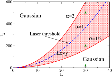
Figure 1: (Color online) Different statistical regimes of fluctuations of a random laser with a two-dimensional slab geometry of thickness $L$. For comparison with the simulations reported below, all quantities are expressed in dimensionless units $\ell=1$, $v=1$. The symbols correspond to the parameters of Fig. 2.

III Numerical Model

In order to provide evidence of the theoretical considerations presented in Section II, we introduce a general, yet easy to simulate, model of random lasing. We consider a sample partitioned in cells of linear size $\ell$. Specifically, we deal with a portion of a two-dimensional square lattice. Thus the center of each cell is identified by the vector index ${\bf r}=(x,y)$, with $x,y$ integers. In the following we will deal with a sample with a slab geometry i.e. $1\leq x\leq L$, $1\leq y\leq RL$. The total number of lattice sites is thus $RL^{2}$ where $R$ defines the slab aspect ratio. Periodic boundary conditions in the $y$ direction are assumed.

Within each cell we have the population $N({\bf r},t)$ of excitations. We consider an hypothetical three–level system with fast decay from the lowest laser level. If the population in the latter can be neglected we can identify $N$ as the number of atoms in the excited state of the lasing transition.

Isotropic diffusion of light is modeled as a standard random walk along the lattice sites. The natural time unit of the dynamics is thus given by $\Delta t=\ell/v$. We choose to describe the diffusion dynamics in terms of a set of $M$ walkers each carrying a given number of photons $n_{1},\ldots n_{M}$. This may be visualized as an ensemble of “beams” propagating independently throughout the sample. Each of their intensities changes in time due to processes of stimulated and spontaneous emission. A basic description of those phenomena can be given in terms of a suitable master equation Carma ; Florescu that would require to take into account the discrete nature of the variables. To further simplify the model we consider that the population and number of photons within each cell are so large for the evolution to be well approximated by the deterministic equations for their averages. In other words, the rate of radiative processes is much larger than that of the diffusive ones and a huge number of emissions occurs within the time scale $\Delta t$ note . With these simplifications $N$ and $n$ can be treated as continuous variables. Altogether the model is formulated by the following discrete–time dynamics:

Step 0: pumping - The active medium is excited homogeneously at the initial time i.e. $N({\bf r},0)=N_{0}$. The value $N_{0}$ represents the pumping level due to some external source. The initial number of walkers is set to $M=0$.

Step 1: spontaneous emission - At each time step and for every lattice site a spontaneous emission event randomly occurs with probability $\gamma N\Delta t$, where $\gamma$ denotes the spontaneous emission rate of the single atom. The local population is decreased by one:

$$N\,\longrightarrow\,N-1\quad,$$ (7)

and a new walker is started from the corresponding site with initial photon number $n=1$. The number of walkers $M$ is increased by one accordingly.

Step 2: diffusion - Parallel and asynchronous update of the photons’ positions is performed. Each walker moves with equal probability to one of its four nearest neighbours. If the boundaries $x=1,L$ of the system are reached, the walker is emitted and its photon number $n_{out}$ recorded in the output. The walker is then removed from the simulation and $M$ is diminished by one.

Step 3: stimulated emission - At each step, the photon numbers $n_{i}$ of each walker and the population are updated deterministically according to the following rules:

$$n_{i}\longrightarrow(1+\gamma\Delta t\,N)\,n_{i}\quad,$$ (8)

$$N\longrightarrow(1-\gamma\Delta t\,n_{i})\,N\quad,$$

where $N$ is the population at the lattice site on which the $i$–th walker resides.

Stochasticity is thus introduced in the model by both the randomness of spontaneous emission events (Step 1) and the diffusive process (Step 2). Note that the model in the above formulation does not include non–radiative decay mechanisms of the population. Furthermore, no dependence on the wavelength is, at present, accounted for; in general $\gamma=\gamma(\lambda)$.

The initialization described in Step 0 is a crude modelling of the pulsed pumping employed experimentally. It amounts to considering an infinitely short excitation during which the samples absorbs $N_{0}$ photons from the pump beam. As a further simplification we also assumed that the excitation is homogeneous throughout the whole sample. More realistic pumping mechanisms can be easily included in this type of modeling. More importantly, as we are going to study the time dependence of the emission, this type of scheme applies to the case in which the time separation between subsequent pump pulses is much larger than the duration of the emitted pulse (i.e. no repumping effects are present).

Steps 1-3 are repeated up to a preassigned maximum number of iterations. The sum of all the photon numbers of walkers flowing out of the medium at each time step is recorded. The resulting time series is binned on a time window of duration $T_{W}$ to reconstruct the output pulse as it would be measured by an external photoncounter. This insures that each point is a sum over a large number of events and makes the comparison with ensemble-averaged results of the preceding Section sensible.

It should be emphasized that, although each walker evolves independently from all the others, they all interact with the same population distribution, which, in turn, determines the photon number distributions. In spite of its simplicity, the model therore describes these two quantities in a self-consistent way.

For convenience, we chose to work henceforth in dimensionless units such that $v=1$, $\ell=1$ (and thus $\Delta t=1$). The only independent parameters are then $\gamma$, the initial population $N_{0}$ (i.e. the pumping level) and the slab sizes $L$, $RL$.

IV Mean–field equations

Before discussing the simulation of the stochastic model it is convenient to present some results on its mean-field limit. When both the population and photon number are large we expect the dynamics to be described by the rate equations for the macroscopic averages. This means that, up to relatively small fluctuations, the individual realization of the stochastic process should follow the solution of Letokhov ; Florescu

$$\dot{N}=-\gamma N(I+1)$$ (9)

$$\dot{I}=D\Delta I+\gamma N(I+1)$$ (10)

where $I(\textbf{r},t)$ is the number of photons in each cell, $\Delta$ denotes the two–dimensional discrete Laplacian and $D=1/4$ in our case.

For simplicity, let us consider the case of a laterally infinite slab ($R\to\infty$) in which both $N$ and $I$ depend on the $y$ coordinate, only. Absorbing boundary conditions are imposed, $I(0,t)=I(L+1,t)=0$. The integration is started from the same initial conditions of the stochastic simulations, namely $N(x,0)=N_{0}$, $I(x,0)=0$.

As a first remark, we note that the threshold condition (5) applies to (10) upon identifying

$$\gamma N_{0}=\frac{1}{\ell_{G}}\quad,\qquad q=\frac{\pi}{L+1}.$$ (11)

We can thus define a critical value of the initial population $N_{c}=Dq^{2}/\gamma$. For $N_{0}<N_{c}$ the total emission is very low being due to spontaneous processes that are only weakly amplified. On the contrary, for $N_{0}>N_{c}$ strong amplification occurs: the number of photons within the sample increases exponentially in time at a rate given by Eq. (5), $r=\gamma N_{0}-Dq^{2}=\gamma(N_{0}-N_{c})$. After the pulse has reached a maximum and the population is depleted, the emission decreases strongly. An estimate of the decay time of the pulse is given by solving the linearized equations around the stationary state $N=0$, $I=0$. A straightforward calculation yields that the long–time evolution is approximated by $N(x,t)=N_{q}(t)\sin(qx)$, $I(x,t)=I_{q}(t)\sin(qx)$ where

$$N_{q}(t)=A\exp(-\gamma t)$$ (12)

$$I_{q}(t)=A\frac{\gamma}{Dq^{2}-\gamma}\exp(-\gamma t)+B\exp(-Dq^{2}t),$$

with $A,B$ being suitable time-independent amplitudes.

The above results have been checked by comparing them with the numerical solution of (10) obtained by simple integration methods of ordinary differential equations. In particular, we checked that both the rise and fall rates of the emission pulses (see the figures in the next section) are consistent with the expected values of $r$ and Eqs. (IV), respectively.

V Monte Carlo simulations

In this Section we report the results of the simulation of the stochastic model. Preliminary runs were performed to check that lasing thresholds exist upon increasing of either the pumping parameter $N_{0}$ and the slab width $L$. The values are in agreement with the theoretical analysis presented above. In addition, checks of relations (2) and (3) have been performed.

As explained in Section III, we monitored the outcoming flux (per unit length) $\phi$ as function of time. The results are compared with the corresponding quantity evaluated from Eqs. (10). In this case, $\phi$ is defined from the discrete continuity equation to be

$$\phi\;=\;\frac{D}{2}\Big{[}I(1,t)+I(L,t)\Big{]}\quad.$$ (13)

The factor 2 comes from taking into account the contribution from the two boundaries $x=0,L$ of the lattice.

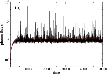
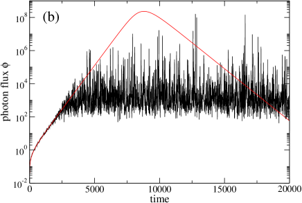
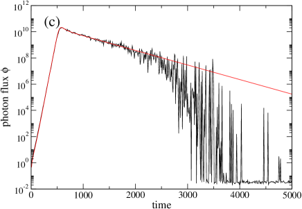
Figure 2: (Color online) The photon flux (per unit length) as a function of time for a single shot, for $N_{0}=2\times 10^{9}$ (a); $N_{0}=5\times 10^{9}$ (b) and $N_{0}=50\times 10^{9}$ (c). Smooth red lines are the mean-field results, evaluated inserting the solutions of Eqs. (10) into Eq. (13). For both curves, data have been binned over consecutive time windows of duration $T_{W}=10$. Note the difference in the vertical–axis scales.

The results of Monte Carlo simulation for a lattice with $L=30$, $R=20$ (18000 sites) and $\gamma=10^{-12}$ (yielding $N_{c}=2.5673\times 10^{9}$) are reported in Fig. 2. The three chosen values of $N_{0}$ are representative of the three relevant statistical regions depicted in Fig. 1: they correspond to $\ell_{G}=500$ (Subthreshold Lévy), $\ell_{G}=200$ (Suprathreshold Lévy) and $\ell_{G}=20$ (Gaussian), respectively (see the triangles in Fig. 1). In the first two cases, the total emission is highly irregular with huge deviations from the expected mean–field behavior. Above the lasing threshold (Fig. 1b) single events (“lucky photons”) may carry values of $n_{i}$ up to $10^{10}$. The resulting time-series are quite sensitive to initialization of the random number generator used in the simulation. On the contrary, in the Gaussian case (Fig. 2c) the pulse is pretty smooth and reproducible, except perhaps for its tails that, however, have a much smaller relative intensity.

The evolution of the population $N$ displays similar features. We have chosen to monitor the volume–averaged population

$$\frac{1}{RL^{2}}\sum_{\textbf{r}}{N(\textbf{r},t)}$$ (14)

normalized to its initial value for a better comparison. Fig. 3 shows the corresponding time–series for the same runs of Fig. 2. Again, large deviations from mean–field appear for the first two values of $N_{0}$. The inset shows that in correspondence with large–amplitude events the population abruptly decreases yielding a distinctive stepwise decay.

The non-smooth time decay is accompanied by irregular evolution in space. Indeed, a snapshot of $N(\textbf{r},t)$ reveals a highly inhomogeneous profile (see Fig. 4). Light regions are traces of high–energy events that locally deplete the population before exiting the sample.

For the Gaussian case, Fig. 2c, similar considerations as those made for the corresponding pulse apply. Note that now the population level decays extremely fast. It reaches 10% of its initial value at $t\approx 600$ which is only twice the average residence time within the sample. This means that photons emitted after a few hundreds time steps have hardly any chance to be significantly amplified (i.e. $\ell_{G}$ has become too large).

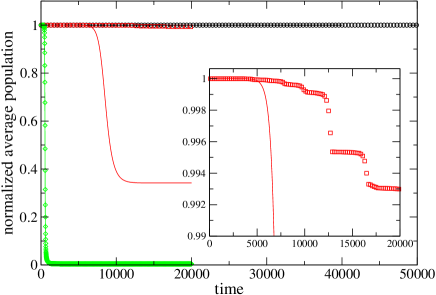
Figure 3: (Color online) The normalized volume-averaged atomic population as a function of time for a single shot and for the same values of $N_{0}$ as in Figs. 2a-c (upper to lower curves respectively). Solid lines are the mean-field results evaluated inserting the solutions of Eqs. (10) into (14). The inset shows a magnification of the middle curves (case $N_{0}=5\times 10^{9}$ of Fig. 2b).

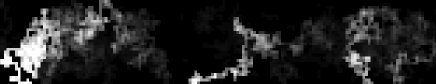
Figure 4: A gray–scale plot of the atomic population distribution along a portion of the lattice for $t=10^{5}$, $N_{0}=5\times 10^{9}$. White regions correspond to small values of $N$.

To check directly the validity of the power–law distribution (4) we computed the histograms of the photon number $n_{out}$ for each and every collected event during the whole simulation run (i.e. the same time range as in Fig. 2). The result are given in Fig. 5 for three values of $N_{0}$ for which the Lévy distribution (4) is expected to occur. A clear power-law tail extending over several decades is observed. Note that the middle curve correspond to the threshold value $N_{0}=N_{c}$ for which we expect $\alpha=1$. Remarkably, the values of the exponents measured by fitting the data are in excellent agreement with the definition of $\alpha$ (see inset of Fig. 5). As predicted, no meaningful value smaller than $\alpha=1/2$ is obtained from the data. It should be noted that we are dealing with a non–stationary process and the results may thus, in principle, depend on the observation time. To check for a possible time-dependence of the statistics, we considered a four-times longer simulation for the case of Fig. 2b and divide the resulting time series in four consecutive parts. Each of the resulting histograms are almost indistinguishable confirming that the underlying process is almost stationary at least on this time scale.

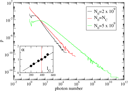
Figure 5: (Color online) Histogram $p(n_{out})$ of the emitted photon numbers $n_{out}$ for the two values of $N_{0}$ of Figs. 2a and b (lower and upper curves) and $N_{0}=N_{c}$ (middle). This middle curve has been vertically shifted for clarity by roughly a factor 5. The inset reports the values of $\alpha$ obtained by a power-law fit of the histograms as a function of the gain length $\ell_{G}$ as defined by Eq. (11). The thin solid line is the theoretical curve as computed by Eqs.  (3) and (4). The dashed vertical line marks the lasing threshold.

Finally, to further elucidate the differences between the two types of statistical regimes, we performed a series of simulations increasing the number of lattice sites. For comparison, we kept $L=30$ fixed and increased the aspect ratio $R$ up to a factor 4. In this way, we increased the number of walkers accordingly. For the Gaussian case, we did observe the expected reduction of fluctuations around the mean–field solution. On the contrary, the wild fluctuations of the Lèvy case were hardly affected. This is a further confirmation of the scenario discussed in Section II.

VI Discussion

Based on heuristic arguments, we have shown in Section II that, depending on the value of the dimensionless parameter ${D\Lambda\ell_{G}}/v$, the fluctuations in the emission of a random laser subject to short pump pulses can be drastically different. In a parameter region extending both above and below threshold, the intensity fluctuations follow a Lévy distribution thus displaying wild fluctuations and huge differences in the emission from pulse to pulse. In the suprathreshold case, such features have been indeed observed in experiments Sharma . Some highly irreproducible emission with lack of self-averaging and very irregular behaviour has been also detected unpub .

The exponent $\alpha$ of the Lévy distribution can be tuned upon changing the pumping level but it must be somehow bounded from below ($\alpha\gtrsim 1/2$) as a further crossover to a Gaussian statistics is attained. Indeed, far above threshold, when the gain length is very small, a large and fast depletion of population occurs (saturation). This hinders the possibility of huge amplification of individual events. In this case all photons behave in a statistically similar way. As a consequence, the statistics is Gaussian and a mean–field description applies again.

The above considerations have been substantiated by comparison with a simple stochastic model. It includes population dynamics in a self–consistent manner. In the Lévy regions, the simulation data strongly depart from the predictions of the mean–field approximation due to the overwhelming role of individual rare events. As a consequence, the evolution of the population displays abrupt changes in time and is highly inhomogeneous in space.

To conclude this general discussion we remark that the width of the Lévy region as defined by inequalities (6) and depicted in Fig. 1 is of order $L^{2}$. Since in our simple model, $\ell_{G}$ is inversely proportional to the pump parameter (see Eq. (11)), the interval of $N_{0}$ values for which the Lévy fluctuations occur shrinks as $1/L^{2}$. Therefore, the larger the lattice, the closer to threshold one must be to observe them.

The existence of different statistical regimes, their crossovers and their dependence on various external parameters enriches the possible experimental scenarios. The emission statistics of random amplifying media has diverging moments in a finite region of parameters extending across the threshold curve. Our theoretical work has shown that, depending on size, geometry, pumping protocols etc., the emission of random lasers may change considerably. This general conclusion should be a useful guidance in understanding past and future experiments on random amplifying media.

References

- (1) P. Sheng, Introduction to Wave Scattering, Localization, and Mesoscopic Phenomena (Academic Press, San Diego, 1995).
- (2) H. Gimperlein et al., Phys. Rev. Lett. 95, 170401 (2005); D. Clement et al., Phys. Rev. Lett. 95, 170409 (2005); C. Fort et al., Phys. Rev. Lett. 95, 170410 (2005).
- (3) V.S. Letokhov, Zh. Éksp. Teor. Fiz. 53, 1442 (1967) [Sov. Phys. JETP 26, 835 (1968)].
- (4) V.M. Markushev, V.F. Zolin, Ch.M. Briskina, Zh. Prikl. Spektrosk. 45, 847 (1986);
- (5) C. Gouedard, et al., J. Opt. Soc. Am. B 10, 2358 (1993).
- (6) N.M. Lawandy, et al., Nature (London) 368, 436 (1994); W.L. Sha, C.H. Liu, and R.R. Alfano, Opt. Lett. 19, 1922, (1994).
- (7) M. Bahoura, K.J. Morris, and M.A. Noginov, Opt. Comm. 201, 405 (2002).
- (8) D.S. Wiersma and S. Cavalieri, Nature 414, 708 (2001).
- (9) D.S. Wiersma and A. Lagendijk, Phys. Rev. E 54, 4256 (1996); Light in strongly scattering and amplifying random systems, D.S. Wiersma (PhD thesis, Univ. of Amsterdam, 1995).
- (10) H. Cao, Y. G. Zhao, S. T. Ho , E. W. Seelig, Q. H. Wang, and R. P. H. Chang, Phys. Rev. Lett. 82, 2278 (1999).
- (11) H. Cao, J. Y. Xu, S.-H. Chang and S. T. Ho, Phys. Rev. E 61, 1985 (2000).
- (12) R.C. Polson, M.E. Raikh, and Z.V. Vardeny, IEEE J. Sel. Topics in Q. Elec. 9, 120 (2003).
- (13) P. Pradhan and N. Kumar, Phys. Rev. B 50, 9644 (1994).
- (14) V. Milner and A.Z. Genack, Phys. Rev. Lett. 94, 073901 (2005).
- (15) S. Mujumdar, M. Ricci, R. Torre, and D. S. Wiersma Phys. Rev. Lett. 93, 053903 (2004).
- (16) A. Yu. Zyuzin, Europhys. Lett. 26, 517 (1994).
- (17) S. John and G. Pang, Phys. Rev. A 54, 3642 (1996).
- (18) L. Florescu and S. John, Phys. Rev. Lett. 93 013602 (2004); Phys. Rev. E 69 046603 (2004)
- (19) B.L. Altshuler, V.E. Kravtsov, and I.V. Lerner, in Mesoscopic Phenomena in Solids, edited by B.L. Altshuler, P.A. Lee, and R.A. Webb (North- Holland, Amsterdam, 1991).
- (20) A. D. Mirlin, Phys. Rep. 326, 259 (2000).
- (21) M. Patra, Phys. Rev. E 67, 016603 (2003).
- (22) V. G. Karpov, Phys. Rev. B 48, 4325 (1993).
- (23) S. E. Skipetrov, and B. A. van Tiggelen, Phys. Rev. Lett. 92, 113901 (2004).
- (24) V. M. Apalkov, M. E. Raikh, and B. Shapiro, Phys. Rev. Lett. 89, 126601 (2002)
- (25) G. A. Berger, M. Kempe and A. Z. Genack, Phys. Rev. E 56 6118 (1997)
- (26) S. Mujumdar, S. Cavalieri and D.S. Wiersma, J. Opt. Soc. Am. B 21 201 (2004).
- (27) X. Jiang and C.M. Soukoulis, Phys. Rev. Lett. 85 70 (2000).
- (28) C.W.J. Beenakker, Phys. Rev. Lett. 81, 1829 (1998).
- (29) D. Anglos et al., J. Opt. Soc. Am. B 21, 208 (2004).
- (30) K. van der Molen, A.P. Mosk, and A. Lagendijk, Phys. Rev. A 74, 053808 (2006).
- (31) D. Sharma, H. Ramachandran and N. Kumar, Fluct. Noise Lett. 6 L95 (2006).
- (32) S. Redner, A Guide to First-passage Processes, (Cambridge University Press, Cambridge, 2001).
- (33) J.P. Bouchaud and A. Georges, Phys. Rep. 195, 127 (1990).
- (34) H.J. Carmichael, Statistical Methods in Quantum Optics 1 (Springer-Verlag, Berlin, 1999).
- (35) In our units this correspond to the condition . For the parameters in the simulations , i.e. the condition may be violated for short times. On the other hand this initial regime is irrelevant for the effects we are interested in.
- (36) S. Mujumdar, V. Tuerck and D.S. Wiersma, unpublished.