Detection of NMR signals with a radio-frequency atomic magnetometer

Abstract

We demonstrate detection of proton NMR signals with a radio frequency atomic magnetometer tuned to the NMR frequency of 62 kHz. High-frequency operation of the atomic magnetometer makes it relatively insensitive to ambient magnetic field noise. We obtain magnetic field sensitivity of 7 fT/Hz^1/2 using only a thin aluminum shield. We also derive an expression for the fundamental sensitivity limit of a surface inductive pick-up coil as a function of frequency and find that an atomic rf magnetometer is intrinsically more sensitive than a coil of comparable size for frequencies below about 50 MHz.

I Introduction

Nuclear magnetic resonance (NMR) signals are commonly detected with inductive radio-frequency (rf) pick-up coils. Recently, alternative detection methods using SQUID magnetometers Mössle et al. (2006); Seton et al. (1997); Greenberg (1998) or atomic magnetometers Yashchuk et al. (2004); Savukov and Romalis (2005) have been explored. These techniques can achieve higher sensitivity at low NMR frequencies and offer other advantages in specific applications. In particular, atomic magnetometers eliminate the need for cryogenic cooling and allow simple multi-channel measurements Kominis et al. (2003). However, most atomic magnetometers are designed to detect quasi-static magnetic fields and are sensitive to oscillating fields only in a limited frequency range. Previous NMR and MRI experiments with atomic magnetometers detected either static nuclear magnetization Newbury et al. (1993); Yashchuk et al. (2004); Xu et al. (2006) or nuclear precession at a very low frequency ($\sim$ 20 Hz) Savukov and Romalis (2005).

Recently we developed an rf atomic magnetometer that can be tuned to detect magnetic fields at any frequency in the kHz to MHz range Savukov et al. (2005) and demonstrated detection of NQR signals at 423 kHz using this device Lee et al. (2006). Another technique for detection of rf fields with atoms is presented in Ledbetter et al. (2006). Here we describe detection of NMR signals from water at 62 kHz and discuss issues specific to NMR detection, such as application of a uniform static magnetic field. The rf magnetometer offers a number of advantages over traditional quasi-static atomic magnetometers. It can detect NMR signals in a wide range of magnetic fields and allows measurements of chemical shifts Saxena et al. (2001). Operation at high frequency reduces the magnetic noise produced by Johnson electrical currents in nearby conductors Varpula and Pautanen (1984). In magnetic resonance imaging applications it increases the available bandwidth and eliminates the effects of transverse magnetic field gradients Meriles et al. (2005). The rf magnetometer also has a number of practical advantages. It is relatively insensitive to changes in DC magnetic field allowing it to operate in an unshielded or lightly shielded environment. Unlike previous setups, we did not use $\mu$-metal magnetic shields in this experiment, relying only on a thin aluminum rf shield. The magnetometer is also relatively insensitive to vibrations and laser noise because it detects alkali-metal spin precession signals at high frequency. We used inexpensive multi-mode diode lasers mounted on an aluminum plate without vibration isolation. We identified several technical issues that need further research, such as improvement in the uniformity of the static magnetic field and reduction of the magnetometer dead time after the rf excitation pulse.

We also compare the fundamental limits on the magnetic field sensitivity for an rf magnetometer and a traditional inductive pick-up coil. We derive an estimate for the sensitivity of a surface pick-up coil over a wide frequency range and compare its optimal performance with that of an atomic rf magnetometer of similar size. We find that the fundamental sensitivity of an atomic magnetometer is higher than fundamental sensitivity of a pick-up coil for frequencies below about 50 MHz.

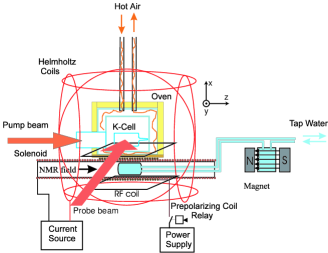
Figure 1: Experimental setup for the observation of water NMR with a radio-frequency atomic magnetometer.

The principle of operation of the rf alkali-metal magnetometer is discussed in Savukov et al. (2005). Briefly, it uses a bias magnetic field to tune the Zeeman resonance frequency of alkali atoms $\nu=\gamma B$ (potassium with nuclear spin $I=3/2$ has $\gamma=g\mu_{B}/\hbar(2I+1)=700$ kHz/Gauss) to the frequency of the oscillating magnetic field. The alkali atoms are optically pumped along the bias field and their transverse spin precession excited by the weak rf field is detected with an orthogonal probe laser. The experimental setup for the magnetometer is shown in Figure 1. Helmholtz coils are used to cancel the Earth field and generate the bias field. The alkali metal is contained in a glass cell that is heated to about 180^∘C with flowing hot air. The sensitivity of the magnetometer near its resonance frequency is shown in Figure 2. The broad peak in the spectral density of the magnetometer signal is due to transverse spin oscillations excited by magnetic field noise and other sources of fluctuations. The width of the peak is equal to the bandwidth of the magnetometer and its height indicates the level of magnetic noise. In Figure 2 we compare the noise levels of the rf magnetometer operating in an unshielded environment, with simple eddy-current shielding using thin aluminum sheets, and inside multi-layer magnetic mu-metal shields. For comparison, with a quasi-static magnetometer operating in an unshielded environment we observed noise of several pT/Hz^1/2 Seltzer and Romalis (2004). The degradation of the performance for an unshielded rf magnetometer is much smaller than for a quasi-static magnetometer and the noise can be further reduced using a more rf-tight aluminum box.

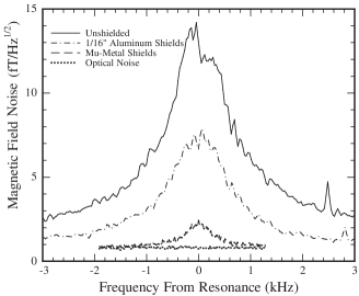
Figure 2: Comparison of sensitivities of high-frequency atomic magnetometer: 1) unshielded (solid line), at 75 kHz; 2) with 1/16” aluminum shield (dash-dotted line), at 75 kHz; 3) mu-metal shielded (dashed line), at 99 kHz; 4) optical noise (dotted line). The NMR signals were detected using the aluminum shield.

For NMR detection the water sample was contained in a 3 cm diameter and 4 cm long cylindrical glass cell. The cell was placed in a solenoid which created a large field inside for the nuclear spins while producing relatively little field outside Yashchuk et al. (2004); Savukov and Romalis (2005). The solenoid is needed to match the resonance frequency of the nuclear spins to the Zeeman resonance of the atomic magnetometer. For efficient detection of the NMR signal the diameter of the solenoid should be close to the diameter of the water sample. At our NMR frequency of 62 kHz the solenoid also needs to have a relatively high magnetic field homogeneity, on the order of $10^{-5}$, to obtain free induction decay time $T_{2}^{*}$ for water close to the intrinsic transverse spin relaxation time. It is relatively easy to make the solenoid long enough or add end-correction coils so that the ends of the solenoid have a negligible effect on the field homogeneity. But we found that near the center of the solenoid the field non-uniformity is limited by variations in the pitch of the winding. Several solenoids were wound on a 3.5 cm OD G10 tube with standard gauge AWG22 magnet wire using different methods, including a lathe with automatic feed control. However, after several winding attempts we were not able to obtain longitudinal field homogeneity better than $1\times 10^{-3}$ over a 3 cm region. The field variation along the axis of the solenoid had a rather random pattern. We suspect the non-uniformity is caused by imperfections in the shape of the wire or non-uniform thickness of enamel insulation. Only a 0.5 $\mu$m variation in the winding pitch is sufficient to explain observed non-uniformity. To improve the field homogeneity we added a short shimming solenoid around the cell which had a variable wire pitch. With appropriate current in the shimming solenoid the field homogeneity along the axis was improved to $1\times 10^{-4}$. However, the improvement in the NMR linewidth was smaller because the shimming solenoid generated large field gradients away from the solenoid axis. The maximum $T_{2}^{*}$ for water NMR signals we were able to obtain was equal to 9 ms at 62 kHz. More work will be needed in the future on the development of magnetic field coils that create highly uniform fields over a large fraction of their volume.

We also investigated in detail the dead time of the atomic magnetometer following an rf pulse needed to tip the nuclear spins. For a simple linear system the dead time is closely related to the bandwidth of the response. As shown in Figure 2, the bandwidth of the atomic magnetometer is on the order of 1 kHz and hence one would expect a dead time on the order of 1 ms. However, for large excitations the response of the rf atomic magnetometer is non-linear. The decay time of the transverse atomic spin oscillations becomes shorter when the longitudinal spin polarization is reduced due to the effect of fast spin-exchange collisions Savukov et al. (2005). Also, because the atomic vapor is optically thick, the propagation of the pumping laser is affected by the degree of atomic spin polarization. If the atoms are completely depolarized during the rf pulse, the time it takes to repump the vapor is proportional to the number of atoms and inversely proportional to the photon flux Bhaskar et al. (1979). In our conditions it takes about 10 ms for the pump laser to polarize the atoms and propagate through the cell.

There are several methods for reducing the dead time of the magnetometer. One can construct a special rf coil Suits and Garroway (2003); Lee et al. (2006) that creates a large magnetic field for the nuclear spins while generating only a small field at the location of the atomic magnetometer. One can temporarily change the bias magnetic field experienced by the atomic magnetometer so the rf pulse is no longer on resonance for the atomic spins and does not cause significant spin excitation Lee et al. (2006). One can also increase the power of the pumping laser to reduce the transverse spin relaxation time - similar to Q-damping techniques used with traditional rf pick-up coils. We have explored the last two techniques here. We verified that the alkali-metal polarization is preserved if the magnetic field is detuned sufficiently far during the rf pulse. It is important that the bias magnetic field is only changed in magnitude, but not in direction, in order not to excite transverse atomic spin oscillations. It is also important to minimize the amount of conductive materials in the vicinity of the magnetometer to reduce eddy currents that prevent quick changes in the bias magnetic field, but this was not easy in our setup. We found that in the existing setup the simplest way to reduce the dead time was by increasing the intensity of the pump laser and reducing the density of alkali-metal atoms. This reduced the repumping time after the rf pulse to about 3 ms but at the same time also reduced the sensitivity of the magnetometer.

To further reduce the effect of dead time, NMR signals were acquired using a spin-echo sequence: a $\pi/2$ pulse followed by a $\pi$ pulse after a time $\tau=15$ msec. The NMR signals were collected in two modes, either using water that was pre-polarized by flowing it through a permanent magnet with a field of 140 mT or using water that was polarized in-situ by a brief application of a 10 mT magnetic field created by a separate pre-polarizing coil wound around the sample. For the flow-through mode the turbulent water motion resulted in an increase of the effective diffusion constant, so successive spin-echo signals had an effective $T_{2}$ decay constant of 140 msec, which resulted in a slight decrease of the signal.

The atomic rf magnetometer is intrinsically sensitive to a magnetic field rotating in the same direction as the alkali-metal atoms Savukov et al. (2005). Nuclear spin precession generates dipolar fields that can be generally decomposed into two counter-rotating components of unequal magnitudes. To obtain the largest NMR signal, the direction of the magnetic field in the solenoid is chosen so the larger of the two rotating NMR field components is co-rotating with the atomic spins.

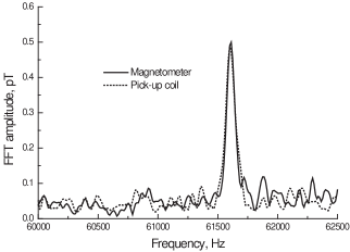
Figure 3: Comparison of the water NMR signal obtained after 10 averages with the rf atomic magnetometer (solid line) and a traditional inductive pick-up coil (dashed line). The water is prepolarized by flow through a 0.14T permanent magnet. Both the atomic magnetometer and the NMR coil are located 5 cm away from the water sample. The active volume of the atomic magnetometer is equal to 0.5 cm³, while the volume of the pick-up coil winding is 19 cm³.

In Figure 3 we show the Fourier transform of the NMR signal detected with the atomic magnetometer compared with the signal detected with a traditional rf pick-up coil, each after 10 averages. In Figure 4 we show the time-domain spin-echo signal obtained with the rf atomic magnetometer after 100 averages. Finally, in Figure 5 we show the NMR signal detected from water that is pre-polarized in-situ by application of a 10 mT magnetic field for 2.5 sec before each spin-echo pulse.

Figure 4: NMR signal from water pre-polarized by flow through an external 0.14 T permanent magnet after 100 averages. The NMR signal is mixed with a reference signal at 60.5 kHz and filtered with bandwidth of 2 kHz. The $\pi/2$ pulse is 0.5 msec long and is applied at $t=0$, the $\pi$ pulse is applied at 12 msec. The recovery time of the magnetometer after the rf pulse is about 3 msec.

Figure 5: FFT of NMR signal after 50 averages from water pre-polarized in-situ by application of a 10 mT magnetic field generated by a small solenoid wound around the water sample. The noise level of the magnetometer under these conditions is 20 fT/Hz^1/2.

It can be seen in Fig. 3 that in our data the signal-to-noise ratio obtained with the atomic magnetometer is comparable to that obtained with a much simpler inductive pick-up coil. Therefore, one can ask under what conditions is the atomic magnetometer advantageous for detection of NMR? To answer this question, we compare the fundamental sensitivity limits for an atomic magnetometer and an inductive pick-up coil. The fundamental sensitivity limit for an atomic magnetometer is derived in Savukov et al. (2005). It is given by

$$\delta B_{at}=\frac{2}{\gamma}\sqrt{\frac{\bar{v}[\sigma_{ex}\sigma_{sd}/5]^{1/2}}{V_{a}}(1+\frac{1}{4\sqrt{\eta}})},$$ (1)

where $\gamma$ is the atomic gyromagnetic factor, $\bar{v}$ is the average thermal velocity, $\sigma_{ex}$ and $\sigma_{sd}$ are the spin-exchange and spin-destruction collision cross sections for alkali atoms, $V_{a}$ is the active volume of the atomic magnetometer and $\eta$ is the quantum efficiency of the photodetectors. The numerical coefficients in Eq.(1) are specific to alkali atoms with nuclear spin $I=3/2$ such as K. In our setup the active volume of the magnetometer is equal to 0.5 cm³ and the fundamental noise limit given by Eq. (1) is equal to 0.14 fT/Hz^1/2, using relaxation cross-sections for K atoms given in Savukov et al. (2005).

Here we derive a relationship for the magnetic field sensitivity of a surface pick-up coil valid in kHz to MHz frequency range. To our knowledge, such general relationship has not been reported previously in the literature. We focus on the surface coil arrangement since for applications using such geometry the coil can be replaced directly with an atomic magnetometer cell. We consider a coil with a mean diameter $D$ and a square winding cross-section of size $W\times W$ with $W\ll D$, as shown in the inset of Fig. 6. First we consider the low frequency limit, where eddy current losses and parasitic capacitance between coil turns can be neglected. Suppose the coil contains $N$ turns of wire with diameter $d$ that fill the available winding volume $V_{w}=\pi DW^{2}$. We ignore small effects due to imperfect filling of the winding volume by circular wire so the number of turns in the coil is $N=4W^{2}/\pi d^{2}$. The voltage induced in the coil by a uniform magnetic field oscillating at frequency $\omega$ is given by $V=B\omega\pi D^{2}N/4$, while the Johnson noise spectral density is given by $V_{n}=\sqrt{16k_{B}T\rho DN/d^{2}}$, where $\rho$ is the resistivity of the wire material, $k_{B}$ is the Boltzman constant and $T$ is the temperature. Combining these relations we get magnetic field sensitivity limited by Johnson noise

$$\delta B_{l}=\frac{8}{\omega D}\sqrt{\frac{k_{B}T\rho}{V_{w}}}.$$ (2)

Thus, ideal sensitivity of an inductive coil scales with the winding volume $V_{w}^{1/2}$, similar to an atomic magnetometer, as well as the frequency and the diameter of the coil. The low frequency limit breaks down for frequencies above a few tens of kHz due to eddy current loses, but Eq. (2) is useful in giving the best possible sensitivity for a pick-up coil.

At higher frequencies we must consider the effects of eddy currents as well as the parasitic capacitance between coil turns. We follow a detailed treatment of the skin depth and proximity effects for circular wires given by Butterworth Butterworth (1921). For a multi-layer coil the total effective AC resistance can be written as

$$R_{ac}=R_{dc}\left(1+F(z)+u(N)\frac{d^{2}}{s^{2}}G(z)\right),$$ (3)

where the next to last and the last terms describe the skin-depth and the proximity effects respectively. The proximity effect is generally larger than the skin-depth effect for multi-turn coils.

The functions $F(z)$ and $G(z)$ are given by the ratio of Bessel functions

$$F(z) = -\frac{z^{2}}{8}{\rm Im}\frac{J_{3}(z\sqrt{-i})}{J_{1}(z\sqrt{-i})},$$

$$G(z) = -\frac{z^{2}}{8}{\rm Im}\frac{J_{2}(z\sqrt{-i})}{J_{0}(z\sqrt{-i})}.$$ (4)

Here $z=d/(\delta\sqrt{2})$, $\delta=(2\rho/\omega\mu_{0})^{1/2}$ is the skin depth of the rf field in the conductor, and $s$ is the spacing between the centers of the wires, $s\geq d$. The function $F(z)$ and $G(z)$ are small for $z<1$ and grow linearly for $z>1$ with the following asymptotic expansions:

$$F(z) = z^{4}/192\,\,\,\,\,\,\,{\rm for}\,\,z<1,$$

$$G(z) = z^{4}/64\,\,\,\,\,\,\,{\rm for}\,\,z<1,$$

$$F(z) = (\sqrt{2}z-3)/4\,\,\,\,\,\,\,{\rm for}\,\,z>3,$$

$$G(z) = (\sqrt{2}z-1)/8\,\,\,\,\,\,\,{\rm for}\,\,z>3.$$ (5)

The function $u(N)$ depends on the winding cross-section and is given by

$$u(N) = \frac{1}{N}\sum_{i=1}^{N}\left[\left(\sum_{j=1,j\neq i}^{N}\frac{x_{j}-x_{i}}{(x_{j}-x_{i})^{2}+(y_{j}-y_{i})^{2}}\right)^{2}\right.$$ (6)

$$+ \left.\left(\sum_{j=1,j\neq i}^{N}\frac{y_{j}-y_{i}}{(x_{j}-x_{i})^{2}+(y_{j}-y_{i})^{2}}\right)^{2}\right],$$

where $x_{i}$ and $y_{i}$ are the positions of the wires in the cross-section of the winding, measured in units of $s$. For a square winding cross-section with uniform wire spacing $u(N)\approx 1.5N$ for $N\gtrsim 20$, while for a circular cross-section $u(N)\rightarrow(\pi/2)N$ for large $N$. For single layer coils, either in the shape of a short solenoid or a flat spiral coil, $u(N)=3.2$ for large $N$.

Since Eq. (2) does not depend on the thickness of the wire, it seems possible to reduce skin effect and proximity effect losses by using a very thin wire and a large number of turns to fill the winding volume $V_{w}$. However, another limitation comes from parasitic capacitance effects. For a multi-layer coil the parasitic capacitance is dominated by the capacitance between layers. We model it by assuming that the coil can be separated into $N_{l}$ winding layers with self-inductance $L_{i}$, resistance $R_{i}$ and parasitic capacitance $C_{i}$ in parallel with each layer Grandi et al. (1999). Each layer has $N_{w}$ wires and $N=N_{w}N_{l}$. For a surface coil geometry with $W\ll D$ the mutual inductance between layers is approximately equal to their self-inductance, $M_{ij}=L_{i}$. For a current $I$ flowing through the coil, the flux through each element $\Phi_{i}=\sum_{j\neq i}M_{ij}I+L_{i}I=N_{l}L_{i}I$. Then the total impendence of the coil is $Z=N_{l}(R_{i}+i\omega N_{l}L_{i})/(1+(R_{i}+i\omega N_{l}L_{i})i\omega C_{i})$. Hence, the coil has a self-resonance frequency given by $\omega_{self}=1/\sqrt{N_{l}L_{i}C_{i}}$.

For a surface coil with $W\ll D$ the self-inductance of each layer is $L_{i}=\mu_{0}DN_{w}^{2}p(D/W)$, where $p(D/W)$ is a slowly varying dimentionless function on the order of unity. The capacitance between layers is approximately given by $C_{i}=\epsilon_{0}\epsilon\pi DW/s$, where $s=W/N_{l}$ is the distance between layers and $\epsilon$ is the relative permeability of the insulation material between wires. Combining these relationships we find the self-resonance frequency $\omega_{self}=c/(DN\sqrt{\pi\epsilon p(D/w)})$, where $c$ is the speed of light. Thus, up to factors of order unity, the self-resonance frequency is determined by the duration of current propagation in the total length of the wire, similar to other types of electromagnetic resonators. In real coils the parasitic capacitance and mutual inductance vary between turns, resulting in significant broadening of the self-resonance. To obtain a high $Q$, coils are always operated significantly below their self-resonance frequency and the number of turns is limited, $N\ll c/D\omega$.

Another common technique for improving coil performance is to use Litz wire made of many strands of very thin wire connected in parallel. This reduces skin effect and proximity effect losses while keeping the total number of turns small. Eddy current losses in Litz wire were also considered by Butterworth in Butterworth (1921). Eq. (3) is slightly modified,

$$R_{ac}=R_{dc}\left(1+F(z)+(u(N)+2)\frac{n^{2}d^{2}}{s^{2}}G(z)\right)$$ (7)

where $n$ is the number of strands in the Litz wire and $d$ is the diameter of each strand, also used for evaluation of $z$. Litz wire is effective for frequencies below a few MHz, at higher frequencies it is not practical to make wire with $d<\delta$.

At higher frequencies one is forced to operate in the regime $d>\delta$ and a simplified equation for the magnetic field sensitivity can be derived using the asymptotic dependence of $F(z)$ and $G(z)$ functions for large $z$,

$$\delta B_{h}=\frac{8}{\omega D}\sqrt{\frac{k_{B}T\rho}{1.8\pi DW\delta}}.$$ (8)

This can be intuitively understood as the modification of Eq. (2) for the case when the current flows only in the surface of the coil winding within a skin depth $\delta$.

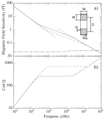
Figure 6: Panel a) Estimated optimal magnetic field sensitivity for a surface pick-up coil with dimensions $D=5$ cm and $W=1$ cm. Solid curve gives the sensitivity for solid wire, while dashed curve is for Litz wire with 1000 strands. The total number of turns and the diameter of the wire is optimized at each frequency. Dotted lines show the asymptotic sensitivity of the coil at low frequency from Eq. (2) and high frequency from Eq. (8). Dot-dashed line shows sensitivity for a K atomic magnetometer occupying the same volume as the coil. Panel b) The $Q$ of the coil with parameters that give optimal sensitivity in panel a). Solid line is for solid wire, dashed line for Litz wire

To estimate the optimal performance for a surface coil we varied the number of turns and the wire diameter for given values of $D$ and a square winding cross-section $W\times W$. We find that other cross-sections, such as a single layer spiral or solenoidal coil with the same winding width $W$ give a worse performance. For a given application the optimal dimensions of the coil are determined by the distance to the sample and its dimensions. The parameters of the coil are optimized subject to constraints that $\omega\leq 0.5\,\omega_{self}$ and the wire diameter (including strand diameter in Litz wire) is greater than 30 $\mu$m. We considered both solid wire and Litz wire with 1000 strands. In Figure 6 we plot the expected magnetic field sensitivity for a surface pick-up coil with $D=5$ cm and $W=1$ cm. We also plot the $Q$ of the coil, showing that the model predicts values of $Q$ that are consistent with or slightly higher than common experimental values of $Q$ for room temperature copper coils, as would be expected for an idealized model. At high frequency $Q$ increases as $f^{1/2}$ Hoult and Richards (1976). It can be seen that the magnetic field sensitivity of a surface coil is well approximated by asymptotic relationships (2) and (8) for frequencies below 30 KHz and above 10 MHz respectively. In the intermediate frequency range the sensitivity is limited by the self-resonance effects or the minimum practical wire diameter. As can be seen in Fig. 6, Litz wire improves magnetic field sensitivity by about a factor of 2 in this regime.

We also plot in Figure 6 the expected optimized sensitivity for an atomic magnetometer occupying the same space as the coil with $V_{a}=\pi(D+W)^{2}W/4$. The atomic magnetometer sensitivity has a slight frequency dependence due to changes in spin-relaxation when the resonance frequency becomes higher than the spin-exchange rate, as discussed in Savukov et al. (2005). We find that a room temperature copper RF coil overtakes the sensitivity of a K magnetometer at approximately 50 MHz.

The model for surface coil sensitivity also gives a good estimate for the sensitivity of the pick-up coil used in our NMR experiment. For detection of NMR signals shown in Figure 3 we used a coil with an average diameter of 3.6 cm, cross-section of 1$\times$1.6 cm², wire diameter $d=0.23$ mm, wire spacing $s=0.5$ mm, and $N=400$. For these parameters, the estimated coil magnetic field sensitivity is about 3 fT/Hz^1/2 at 66 kHz, close to the optimum for given coil dimensions. This theoretical estimate is in a good agreement with actual magnetic noise measurements when the pick-up coil was placed in a well-shielded aluminum box. When the coil was used in the NMR setup, the measured noise level was 7 fT/Hz^1/2, equal to the noise level measured by the atomic magnetometer under the same shielding conditions. Thus, it is not surprising that the noise level in Figure 3 is the same for the atomic magnetometer and the pick-up coil, both being limited by external noise sources. With better eddy-current shielding or by using a gradiometric measurement Kominis et al. (2003) one can expect to significantly reduce the noise of the atomic magnetometer while the pick-up coil is already operating near the fundamental limit of its sensitivity.

It is also interesting to compare the sensitivity of an rf atomic magnetometer with that of a SQUID magnetometer. While at low frequencies SQUID detectors typically have sensitivity of about 1 fT/Hz^1/2, at frequencies above a few kHz a tuned superconducting resonator can be used to improve their performance  Seton et al. (1997, 2005). For example, magnetic field sensitivity of 0.035 fT/Hz^1/2 has been demonstrated at 425 kHz using a 5-cm diameter superconducting pick-up coil and a resonator with $Q=10^{5}$ Seton et al. (2005). Atomic magnetometers have not yet experimentally reached this level of sensitivity, although it is possible based on fundamental sensitivity limits given by Eq. (1). On the other hand, they have a larger bandwidth, which is important for many applications. For example, in Lee et al. (2006) magnetic field sensitivity of 0.24 fT/Hz^1/2 has been demonstrated for an rf atomic magnetometer with $Q$ of $10^{3}$ at 423 kHz.

In conclusion, we have demonstrated the first detection of proton NMR signals with an rf atomic magnetometer. The advantages of this technique include relative insensitivity of the rf magnetometer to ambient magnetic field noise and the possibility of measuring NMR chemical shifts. We also demonstrated in-situ prepolarization of proton spins, opening the possibility of efficient magnetic resonance imaging with an atomic magnetometer that does not rely on remote encoding Xu et al. (2006). We identified several issues that need further improvements, such as better magnetic field homogeneity for compact solenoids and more efficient damping of magnetometer spin transients. Finally, we derived a simple relationship for estimating the magnetic field sensitivity of a surface coil over a wide frequency range. Comparing it with that of an atomic magnetometer we find that atomic magnetometers have an intrinsic sensitivity advantage over a pick-up coil for frequencies below about 50 MHz. Thus, they are well-suited for detection of NQR signals as well as for low field NMR and MRI.

We like to thank K. Sauer for helpful discussions. This work was supported by the NSF and the Packard Foundation.

References

- Mössle et al. (2006) M. Mössle, W. R. Myers, S.-K. Lee, N. Kelso, M. Hatridge, A. Pines, and J. Clarke, IEEE Transactions on Applied Superconductivity 15, 757 (2006).
- Greenberg (1998) Y. S. Greenberg, Rev. Mod. Phys. 70, 175 (1998).
- Seton et al. (1997) H. C. Seton, J. M. S. Hutchison, and D. M. Bussell, IEEE Trans. Appl. Supercond. 7, 3213 (1997).
- Yashchuk et al. (2004) V. V. Yashchuk, J. Granwehr, D. F. Kimball, S. M. Rochester, A. H. Trabesinger, J. T. Urban, D. Budker, and A. Pines, Phys. Rev. Lett. 93, 160801 (2004).
- Savukov and Romalis (2005) I. M. Savukov and M. V. Romalis, Phys. Rev. Lett. 94, 123001 (2005).
- Kominis et al. (2003) I. K. Kominis, T. W. Kornack, J. C. Allred, and M. V. Romalis, Nature 422, 596 (2003).
- Newbury et al. (1993) N. R. Newbury, A. S. Barton, P. Bogorad, G. D. Cates, M. Gatzke, H. Mabuchi, and B. Saam, Phys. Rev. A 48, 558 (1993).
- Xu et al. (2006) S. Xu, V. Yashchuk, M. Donaldson, S. Rochester, D. Budker, and A. Pines, Proc. Nat. Acad. Sci. USA 103, 12668 (2006).
- Savukov et al. (2005) I. M. Savukov, S. J. Seltzer, M. V. Romalis, and K. L. Sauer, Phys. Rev. Lett. 95, 063004 (2005).
- Lee et al. (2006) S.-K. Lee, K. L. Sauer, S. J. Seltzer, O. Alem, and M. V. Romalis, Appl. Phys. Lett (in press) (2006).
- Ledbetter et al. (2006) M. P. Ledbetter, V. M. Acosta, S. M. Rochester, D. Budker, S. Pustelny, and V. V. Yashchuk, physics/0609196 (2006).
- Saxena et al. (2001) S. Saxena, A. Wong-Foy, A. J. Moule, J. A. Seeley, R. McDermott, J. Clarke, and A. Pines, J. Am. Chem. Soc. 123, 8133 (2001).
- Varpula and Pautanen (1984) T. Varpula and T. Pautanen, J. Appl. Phys. (1984).
- Meriles et al. (2005) C. A. Meriles, D. Sakellariou, A. H. Trabesinger, V. Demas, and A. Pines, PNAS 102, 1840 (2005).
- Seltzer and Romalis (2004) S. J. Seltzer and M. V. Romalis, Appl. Phys. Lett. 85, 4804 (2004).
- Bhaskar et al. (1979) N. D. Bhaskar, M. Hou, B. Suleman, and W. Happer, Phys. Rev. Lett. 43, 519 (1979).
- Suits and Garroway (2003) B. H. Suits and A. N. Garroway, J. Appl. Phys. 94, 4170 (2003).
- Butterworth (1921) S. Butterworth, Phil. Trans. Roy. Soc. Lon. A222, 57 (1921).
- Grandi et al. (1999) G. Grandi, M. K. Kazimierczuk, A. Massarini, and U. Reggiani, IEEE Transactions of Industry Applications 35, 1162 (1999).
- Hoult and Richards (1976) D. Hoult and R. Richards, J. of Magn. Res. 24, 71 (1976).
- Seton et al. (2005) H. Seton, J. Hutchison, and D. Bussell, Cryogenics 45, 348 (2005).