Penrose-Carter diagram for an uniformly accelerated observer

Abstract

An uniformly accelerated observer can build his proper system of coordinates in a delimited sector of the flat Minkowski spacetime. The properties of the position and time coordinate lines for such an observer are studied and compared with the coordinate lines for an inertial observer in a Penrose-Carter diagram for this spacetime.

I Introduction

It is sometimes useful to dispose of a graphical representation of the totality of the spacetime, for instance to study asymptotic forms of various fields (metric, curvature tensor, electromagnetic field, etc.). A very elegant mathematical technique to study the asymptotic properties of spacetimes has been developed simultaneously by Roger Penrose and Brandon Carter penr64 ; hawk73 . The idea is to perform what is called a conformal transformation of spacetime to bring infinities at finite distances while preserving its causal structure (light cones are unaltered). Asymptotic calculations are then converted into calculations at finite points with a set of new coordinates, the conformal coordinates, which attribute finite values to infinities. Thereby, a global picture of the causal structure for the totality of the studied spacetime can be more easily obtained. The diagram of the spacetime after transformation is called a Penrose-Carter diagram.

Students are sometimes confronted for the first time with Penrose-Carter diagrams by studying the spacetime around a static or a rotating black hole. Even if the flat Minkowski spacetime is studied with conformal coordinates, exact coordinate line equations are often not given and their properties are rarely studied. The purpose of this paper is to perform a detailed study with conformal coordinates of the simplest possible spacetime, the flat Minkowski spacetime, from the point of view of an inertial observer and an uniformly accelerated observer. The conformal coordinates and the proper coordinates of the uniformly accelerated observer are both obtained from a change of coordinates. But, these two transformations have different physical contents which will discussed within the text.

The intrinsic properties of a spacetime cannot depend on the system of coordinates used to map this spacetime. But, a better understanding of the structure of a spacetime can be obtained by the knowledge of its coordinate lines with a clear physical meaning. A natural choice is to take, when it is possible, lines with constant time or position. For the flat Minkowski spacetime, these coordinate lines are straight lines cutting each other at right angle in an ordinary diagram while, in a Penrose-Carter diagram, the equations of these lines are complicated functions of the conformal coordinates. These are studied in section II.

The motion of an observer with a constant proper acceleration can be treated analytically. It is a classical exercise of special relativity that can be found in many textbooks sear68 ; misn73 ; rind77 ; sema05 . In this framework, the very prominent notion of event horizon can be introduced in a simpler context than the one of black hole for instance. An uniformly accelerated observer can build his proper system of coordinates in a delimited, but infinite, sector of the flat Minkowski spacetime rind66 ; desl87 ; desl89 ; frol98 ; sema06 . The corresponding time and position coordinate lines are respectively hyperbolas and straight lines in an ordinary diagram. A detailed study of the equations of these lines with conformal coordinates is performed in section III.

A brief summary of our results about these mappings of the flat Minkowski spacetime for both an inertial observer and an uniformly accelerated observer is given in section IV.

Penrose-Carter diagrams are generally used with spatial spherical coordinates plus a time coordinate. In this case, the study of only radial trajectories of particles, with angular coordinates fixed, is performed in a $1+1$ Minkowski spacetime. In this paper, we will consider rectangular coordinates plus a time coordinate. As we will look only at motions along the $x$-axis, keeping $y$ and $z$ coordinates fixed, all results are also presented in a $1+1$ Minkowski spacetime.

II The Minkowski spacetime

II.1 Change of coordinates

The usual change of coordinates to bring back infinities at finite distances is

$$ct+x = L\tan(\psi+\xi),$$

$$ct-x = L\tan(\psi-\xi),$$ (1)

with $-\pi/2<\psi\pm\xi<\pi/2$. $L$ is an arbitrary length, and $\psi$ and $\xi$ are dimensionless quantities, the conformal coordinates. It is useful to define new dimensionless spacetime variables: $T=ct/L$ and $X=x/L$ which will be used throughout the text. Equations (II.1) are then reduced to

$$T+X = \tan(\psi+\xi),$$

$$T-X = \tan(\psi-\xi).$$ (2)

With these conformal coordinates, the totality of the spacetime is represented by a square (see figure 1), sometimes called the “Minkowski diamond”. As we will see below, coordinate lines with constant position and time converge at the apexes of the square. These points are the conformal infinities for space and time.

The equation of motion of a photon passing by the position $X_{*}$ at time $T_{*}$ is $X\pm T=X_{*}\pm T_{*}$. In the conformal coordinates, it is written

$$\xi\pm\psi=\arctan(X_{*}\pm T_{*}).$$ (3)

So, as in an ordinary diagram, the world line of a photon in the Penrose-Carter diagram is still a line slanted at an angle of 45^∘, but with respect to the $\xi$ and $\psi$ coordinates. The causal structure in the Penrose-Carter diagram is given by light cones for variables $\xi$ and $\psi$, as it is given by light cones for variables $X$ and $T$ in an ordinary diagram. The diagonal boundaries of the Penrose-Carter diagram are the infinities where world line of light rays must end.

With the new coordinates, the metric $ds^{2}=c^{2}dt^{2}-dx^{2}$ is written

$$ds^{2}=L^{2}(dT^{2}-dX^{2})=L^{2}\frac{d\psi^{2}-d\xi^{2}}{\cos^{2}(\psi+\xi)\cos^{2}(\psi-\xi)}.$$ (4)

II.2 Coordinate lines

Following equations (II.1), a time coordinate line with the constant position $X_{*}$ is given by

$$2X_{*}=\tan(\psi+\xi)-\tan(\psi-\xi).$$ (5)

Using the properties of the tangent function, this relation can be recast into the form

$$\xi(\psi,X_{*})=\arctan\left[\frac{-(1+\tan^{2}\psi)+\sqrt{(1+\tan^{2}\psi)^{2}+4X_{*}^{2}\tan^{2}\psi}}{2X_{*}\tan^{2}\psi}\right],$$ (6)

with $\psi\in\ ]-\pi/2,\pi/2[$ and $X_{*}\in\ ]-\infty,\infty[$ (see figure 1). This function is even for the variable $\psi$ and odd for the variable $X_{*}$. It is vanishing at the conformal time infinities, $\xi(\pm\pi/2,X_{*})=0$, and $\xi(0,X_{*})=\arctan X_{*}$.

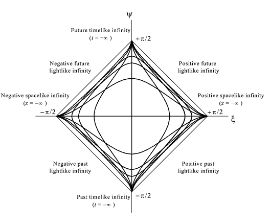
Figure 1: Coordinate lines for the Minkowski spacetime in the Penrose-Carter diagram. From left to right, lines for constant positions $X_{*}=-3,-2,-1,0,1,2,3$ are indicated. From bottom to top, lines for constant times $T_{*}=-3,-2,-1,0,1,2,3$ are indicated. The $X_{*}=0$ ($T_{*}=0$) line is the $\xi$=0 ($\psi=0$) line.

The derivative of function (6) with respect to $\psi$ is written

$$\partial_{\psi}\xi(\psi,X_{*})=\frac{-\sqrt{2}X_{*}\sin(2\psi)}{\sqrt{2+X_{*}^{2}(1-\cos(4\psi))}}.$$ (7)

It has three zeros for all values of $X_{*}$: $\partial_{\psi}\xi(\pm\pi/2,X_{*})=\partial_{\psi}\xi(0,X_{*})=0$. The slopes at extremities of these coordinate lines are then vanishing.

For infinite values of $X_{*}$, we obtain

$$\lim_{X_{*}\to\pm\infty}\xi(\psi,X_{*})=\pm\arctan\left(|\cot\psi|\right),$$ (8)

that is to say, $\xi=\pm(\psi+\pi/2)$ for $\psi\in[-\pi/2,0]$ and $\xi=\pm(\pi/2-\psi)$ for $\psi\in[0,\pi/2]$. These are the boundaries of the spacetime, as expected. Let us note that we have

$$\lim_{X_{*}\to\pm\infty}\partial_{\psi}\xi(\psi,X_{*})=\left\{\ \begin{array}[]{l}\phantom{-}0\ \textrm{for}\ \psi=-\pi/2,0,\pi/2\\ \pm 1\ \textrm{for}\ \psi\in\ ]-\pi/2,0[\\ \mp 1\ \textrm{for}\ \psi\in\ ]0,\pi/2[\end{array}\right.,$$ (9)

in agreement with the results given just above.

A space coordinate line with the constant time $T_{*}$ is given by

$$2T_{*}=\tan(\psi+\xi)+\tan(\psi-\xi).$$ (10)

The transformations $T_{*}\leftrightarrow X_{*}$ and $\psi\leftrightarrow\xi$ change this equation into equation (5). So there is a complete symmetry between time and space coordinate lines, as expected. Their properties are the same and the discussion above can be completely adapted to the space coordinate lines.

III The uniformly accelerated observer

III.1 Hyperbolic motion

Let us consider an uniformly accelerated observer with a constant proper acceleration with magnitude $A>0$. Its motion is such that it reaches the point $x=0$ in the inertial frame at time $t=0$ with a vanishing speed. The world line of the observer is given by sear68 ; misn73 ; rind77 ; sema05 ; rind66 ; desl87 ; desl89 ; frol98 ; sema06

$$\left(\frac{A\,x}{c^{2}}+1\right)^{2}-\left(\frac{A\,ct}{c^{2}}\right)^{2}=1,$$ (11)

which is the equation of a branch of hyperbola in spacetime. So this motion is also called hyperbolic.

If we choose $L=c^{2}/A$, this equation can be recast into the form

$$\left(X+1\right)^{2}-T^{2}=1.$$ (12)

The asymptotes of this curve are the two straight lines with equations $T=\pm(X+1)$. Consequently, the asymptotes of the world line of the accelerated observer defines two event horizons sear68 ; misn73 ; rind77 ; sema05 ; rind66 ; desl87 ; desl89 ; frol98 ; sema06 . In the conformal coordinates, equations of these horizons are

$$\psi=\pm(\xi+\pi/4).$$ (13)

These two horizons cross at event $H$ with spacetime coordinates $(\xi_{H},\psi_{H})=(0,-\pi/4)$ corresponding to $(X,T)=(-1,0)$. The past (future) horizon intercepts the positive past (future) light infinity at event $S$ ($E$) with spacetime coordinates $(\xi_{S},\psi_{S})=(\pi/8,-3\pi/8)$ ($(\xi_{E},\psi_{E})=(\pi/8,3\pi/8)$). They cut the whole spacetime in four regions, called Rindler sectors (see figure 2) frol98 . The sector I is the portion of the spacetime in which the uniformly accelerated observer lives: he can send information to any event and he can receive information from any event in this sector. In sector II, located “above” the future horizon, the observer can send information to any event but cannot receive information from this sector. The situation is exactly the opposite in the sector IV, located “below” the past horizon. The sector III is causally completely disconnected from the observer.

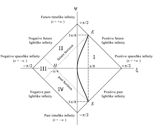
Figure 2: World line of the uniformly accelerated observer in the Penrose-Carter diagram for the Minkowski spacetime. Past and future event horizons are indicated with the four Rindler sectors.

Written in the conformal coordinates, equation (12) becomes

$$-\tan(\psi+\xi)\tan(\psi-\xi)+\tan(\psi+\xi)-\tan(\psi-\xi)=0.$$ (14)

This relation can be recast into the form

$$\xi=\arctan\left[-(1+\tan^{2}\psi)+\sqrt{(1+\tan^{2}\psi)^{2}+\tan^{2}\psi}\right].$$ (15)

One can check that this world line starts at the event $S$ and ends at the event $E$, both on positive lightlike infinity, as expected since the speed of this observer is equal to the speed of light in the infinite past and future.

The uniformly accelerated observer can build his proper system of dimensionless coordinates, spacelike $X_{0}$ and timelike $T_{0}$, valid only in sector I rind66 ; desl87 ; desl89 ; frol98 ; sema06 . The change of coordinates between $(T,X)$ and $(T_{0},X_{0})$ is given by sema06

$$T=(X_{0}+1)\sinh T_{0},$$

$$X+1=(X_{0}+1)\cosh T_{0}.$$ (16)

The corresponding metric is

$$ds^{2}=L^{2}\left[(X_{0}+1)^{2}dT_{0}^{2}-dX_{0}^{2}\right].$$ (17)

With relations (16), it is possible to determine, in the inertial frame, the equations of the coordinate lines of this observer proper frame. In this last frame, the equation of a time coordinate line with $X_{0}$ constant is

$$\left(X+1\right)^{2}-T^{2}=\left(X_{0}+1\right)^{2}.$$ (18)

This curve is a branch of hyperbola whose asymptotes are the two event horizons mentioned above. These horizons are located on the degenerate asymptotes obtained with $X_{0}=-1$ in equation (18). Obviously, the world line of the uniformly accelerated observer in his proper frame is given by $X_{0}=0$. Let us note that an object with a constant position $X_{0}$ is not at rest with the uniformly accelerated observer. This object is characterized by a proper uniform acceleration whose magnitude $A(X_{0})$ is given by desl89 ; sema06

$$A(X_{0})=\frac{A}{1+X_{0}}.$$ (19)

In the same way, the distance between the uniformly accelerated observer and an object with the same proper acceleration $A$ varies exponentially with the proper time of the observer sema06 .

The equation of a position coordinate line with $T_{0}$ constant is

$$T=\left(X+1\right)\tanh T_{0}.$$ (20)

This is a straight line containing the event $(X,T)=(-1,0)$, that is to say the event $H$, the intersection of the two event horizons. Some coordinate lines are drawn in figure 3. It can be seen that the future horizon and the past horizon correspond respectively to the position coordinate lines $T_{0}=+\infty$ and $T_{0}=-\infty$. Both horizons form also the space coordinate line $X_{0}=-1$.

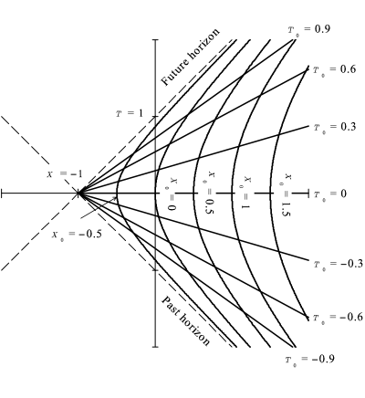
Figure 3: Coordinate lines, associated with an uniformly accelerated observer, for constant times $T_{0}$ (straight lines) and for constant positions $X_{0}$ (hyperbolas), in an inertial frame. The world line of the observer is the coordinate line $X_{0}=0$.

Transformations (II.1) and (16) are both changes of coordinates from the usual coordinates $(T,X)$ defined in the inertial frame of the flat Minkowski spacetime. But, their physical content is strongly different.

With the change of coordinates (II.1), bringing back infinities at finite distances, the coordinates lines are heavily distorted but the coordinates $(\psi,\xi)$ are just another set of coordinates for the inertial observer in the whole flat Minkowski spacetime, with the particularity that light cones are preserved. To some extent, the distortions produced in the transformation $(T,X)\rightarrow(\psi,\xi)$ are like those obtained for the transformation in the plane passing from Cartesian coordinates $(x,y)$ to polar coordinates $(r,\theta)$: A straight line $y=ax+b$ in the plane is generally not represented by a straight line in a $(r,\theta)$ diagram.

The coordinates $(T_{0},X_{0})$, coming from the change of coordinates (16), are the proper coordinates in the non inertial frame of an uniformly accelerated observer and are only valid in a limited sector of spacetime. For this observer, all objects in free motion in the Minkowski spacetime undergo an accelerated motion and the light ray world lines are given by exponential functions desl87 . The uniformly accelerated observer has the impression that an uniform gravitational field exists in his surroundings, although the spacetime is in reality always flat desl89 .

Now, we will express the coordinate lines (18) and (20) with the conformal coordinates in order to draw them in the Penrose-Carter diagram. In the calculations, the following two identities will be useful:

$$\tan\frac{\pi}{8}=\sqrt{2}-1\quad\textrm{and}\quad\tan\frac{3\pi}{8}=\sqrt{2}+1.$$ (21)

III.2 Position coordinate lines

With the conformal coordinates, equation (20) is given by

$$\tan(\psi+\xi)+\tan(\psi-\xi)=\tanh T_{0}\left[\tan(\psi+\xi)-\tan(\psi-\xi)+2\right].$$ (22)

After some calculations, the position coordinate line equation, with $T_{0}$ constant, for the uniformly accelerated observer (uao) can be written

$$\psi_{\textrm{uao}}(\xi,T_{0})=\arctan\left[\frac{1+\tan^{2}\xi-\sqrt{(1+\tan^{2}\xi)^{2}-4\tanh^{2}T_{0}\tan\xi(1-\tan^{2}\xi)}}{2\tanh T_{0}\tan\xi(1-\tan\xi)}\right],$$ (23)

with $\xi\in\ ]-\pi/4,\pi/2[$ and $T_{0}\in\ ]-\infty,\infty[$ (see figure 4). This function is vanishing at the two spacelike extremities of sector I, $\psi_{\textrm{uao}}(-\pi/4,T_{0})=\psi_{\textrm{uao}}(\pi/2,T_{0})=0$. It is odd for the variable $T_{0}$ and, obviously, we have $\psi_{\textrm{uao}}(\xi,0)=0$. The position coordinate line with $T_{0}=0$ cuts sector I in two equal parts. We can expect that $\psi_{\textrm{uao}}$ is even for the variable $\xi$ with respect to $\pi/8$, the middle of the interval $]-\pi/4,\pi/2[$. If we define the new variable $y=\xi-\pi/8$, it can be checked, after a tedious calculation, that $\psi_{\textrm{uao}}(y,T_{0})=\psi_{\textrm{uao}}(-y,T_{0})$. We can compute that $\psi_{\textrm{uao}}(\pi/8,T_{0})=\arctan\left[(1+\sqrt{2})\tanh\frac{T_{0}}{2}\right]$, which implies that $\lim_{T_{0}\to\pm\infty}\psi_{\textrm{uao}}(\pi/8,T_{0})=\pm 3\pi/8$; the two timelike infinities of sector I are reached.

The derivative of function (23) with respect to $\xi$ is given by

$$\partial_{\xi}\psi_{\textrm{uao}}(\xi,T_{0})=\frac{\cos^{2}\xi\tanh T_{0}\left(1-\tan\xi(2+\tan\xi)\right)}{\sqrt{1-\sin(4\xi)\tanh^{2}T_{0}}}.$$ (24)

Due to the symmetry properties of the position coordinate lines, we have $\partial_{\xi}\psi_{\textrm{uao}}(\pi/8,T_{0})=0$. But, at the two spacelike extremities of sector I, the derivatives are not vanishing and varies between $-1$ and $1$: $\partial_{\xi}\psi_{\textrm{uao}}(-\pi/4,T_{0})=\tanh T_{0}$ and $\partial_{\xi}\psi_{\textrm{uao}}(\pi/2,T_{0})=-\tanh T_{0}$. When $T_{0}\to\pm\infty$, the position coordinate lines form the edges of sector I.

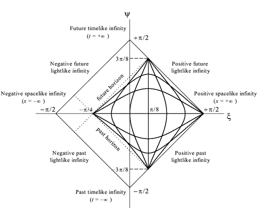
Figure 4: Coordinate lines associated with the uniformly accelerated observer, for constant times $T_{0}$ and for constant positions $X_{0}$, in the Penrose-Carter diagram for the Minkowski spacetime. From bottom to top, constant time lines for $T_{0}=-1,-0.5,0,0.5,1$ are indicated. From left to right, constant position lines for $X_{0}=\tan\frac{s\pi}{8}$ with $s=-1,0,1,2,3$ are indicated. The $T_{0}=0$ line is the $\psi=0$ line. The world line of this observer is the coordinate line $X_{0}=0$.

III.3 Time coordinate lines

With the conformal coordinates, equation (18) is given by

$$-\tan(\psi+\xi)\tan(\psi-\xi)+\tan(\psi+\xi)-\tan(\psi-\xi)=Y_{0},$$ (25)

with $Y_{0}=X_{0}(X_{0}+2)$. After some calculations, the time coordinate line equation, with $X_{0}$ constant, can be written

$$\xi_{\textrm{uao}}(\psi,X_{0})=\arctan\left[\frac{-(1+\tan^{2}\psi)+\sqrt{(1+\tan^{2}\psi)^{2}+(1+Y_{0}\tan^{2}\psi)(Y_{0}+\tan^{2}\psi)}}{1+Y_{0}\tan^{2}\psi}\right].$$ (26)

with $\psi\in\ ]-3\pi/8,3\pi/8[$ and $X_{0}\in\ ]-1,\infty[$ (see figure 4). This function is even for the variable $\psi$. Since $\xi_{\textrm{uao}}(0,X_{0})=\arctan X_{0}$, we have $\lim_{X_{0}\to-1}\xi_{\textrm{uao}}(0,X_{0})=-\pi/4$ and $\lim_{X_{0}\to\infty}\xi_{\textrm{uao}}(0,X_{0})=\pi/2$; the two spacelike infinities of sector I are reached. Because $\xi_{\textrm{uao}}(\pm 3\pi/8,X_{0})=\pi/8$, the coordinate lines (26) connect the two events $S$ and $E$, the timelike infinities of sector I.

The derivative of function (26) with respect to $\xi$ is given by

$$\partial_{\psi}\xi_{\textrm{uao}}(\psi,X_{0})=\frac{\left(1-Y_{0}\right)\tan\psi}{\sqrt{\sec^{4}\psi+(1+Y_{0}\tan^{2}\psi)(Y_{0}+\tan^{2}\psi)}}.$$ (27)

As expected from the symmetry properties of the position coordinate lines, we have $\partial_{\psi}\xi_{\textrm{uao}}(0,T_{0})=0$. But, at the two timelike extremities of sector I, the derivatives are not vanishing and varies between $-1$ and $1$:

$$\partial_{\psi}\xi_{\textrm{uao}}(\pm 3\pi/8,X_{0})=\pm p(X_{0})\quad\textrm{with}\quad p(X_{0})=\frac{1-X_{0}(X_{0}+2)}{3+X_{0}(X_{0}+2)}.$$ (28)

We have $\lim_{X_{0}\to-1}p(X_{0})=1$ and $\lim_{X_{0}\to\infty}p(X_{0})=-1$. When the position $X_{0}$ reaches its extremal values, the time coordinate lines form also the edges of sector I.

We can also remark that $p(\tan\frac{\pi}{8})=0$, and it can be shown that $\xi_{\textrm{uao}}(\psi,\tan\frac{\pi}{8})=\pi/8$. We can wonder if $\xi_{\textrm{uao}}$ is odd for the variable $X_{0}$ with respect to $\tan\frac{\pi}{8}$. If we define the new variable $u$ with $X_{0}=\tan(\frac{\pi}{8}-u)$ and the new function $w$ by $\xi_{\textrm{uao}}=\pi/8-w$, it can be checked, after a tedious calculation, that $w(u)$ is an odd function of $u$. The time coordinate line with $X_{0}=\tan\frac{\pi}{8}$ cuts sector I in two equal parts.

III.4 Link between coordinate lines

By looking at figure 4, it seems that the position and time line coordinates are very similar. So we can study the differences between the functions $\xi_{\textrm{uao}}(a,X_{0})-\pi/8$ and $\psi_{\textrm{uao}}\left(a+\pi/8,T_{0}\right)$ with $a\in\ ]-3\pi/8,3\pi/8[$. Suitable translations are made in order that both functions coincide at their extremities: $a=\pm 3\pi/8$. To perform a comparison, a link must be found between variables $X_{0}$ and $T_{0}$. Knowing the domain of each of these quantities, we can try

$$T_{0}(X_{0})=\arg\tanh\left[\frac{8}{3\pi}\left(\arctan X_{0}-\frac{\pi}{8}\right)\right].$$ (29)

We have then $T_{0}(X_{0}=-1)=-\infty$, $T_{0}(X_{0}=\tan\frac{\pi}{8})=0$ and $T_{0}(X_{0}=\infty)=\infty$.

Let us define the two new functions

$$f_{T}(a,b) = \xi_{\textrm{uao}}(a,b)-\frac{\pi}{8},$$ (30)

$$f_{X}(a,b) = \psi_{\textrm{uao}}\left(a+\frac{\pi}{8},T_{0}(b)\right),$$ (31)

with $a\in\ ]-3\pi/8,3\pi/8[$ and $b\in\ ]-1,\infty[$. Thanks to equation (29), these functions are built in such a way that $f_{T}(a,b)-f_{X}(a,b)$ is vanishing for all values of $a$ when $b=-1$, $\tan\frac{\pi}{8}$ and $\infty$, that is to say when the corresponding coordinate lines form the borders of sector I and when they cut symmetrically this sector. As $f_{T}(\pm 3\pi/8,b)=f_{X}(\pm 3\pi/8,b)=0$ and as these functions are even in $a$, we define the maximal relative gap $\Delta$ between $f_{T}$ and $f_{X}$ by the formula

$$\Delta(b)=2\frac{f_{T}(0,b)-f_{X}(0,b)}{f_{T}(0,b)+f_{X}(0,b)}.$$ (32)

We can see on figure 5 that the gap is always small. We could expect that $\Delta(\tan\frac{\pi}{8})=0$, but this not the case because $f_{T}(0,\tan\frac{\pi}{8})=f_{X}(0,\tan\frac{\pi}{8})=0$. We can also remark that $\Delta(0)=\Delta(1)=0$. Actually, it is possible to show, after some lengthy calculations, that $f_{T}(a,b)=f_{X}(a,b)$ when $b=0$ and 1, for all values of $a$. Finally, we have $\xi_{\textrm{uao}}(a,X_{0})-\pi/8=\psi_{\textrm{uao}}(a+\pi/8,T_{0})$ for $(X_{0},T_{0})=(-1,-\infty)$, $(0,-\arg\tanh\frac{1}{3})$, $(\tan\frac{\pi}{8},0)$, $(1,\arg\tanh\frac{1}{3})$ and $(\infty,\infty)$.

Figure 5: Maximal relative gap $\Delta$ (see formula (32)) as a function of $X_{0}$.

IV Summary

In this paper, a detailed study of the simplest possible spacetime, the flat Minkowski spacetime, is performed with conformal coordinates, from the point of view of an inertial observer and an uniformly accelerated observer. Equations for coordinate lines with constant time or position are given and their properties are studied.

Transformations (II.1) and (16) are both possible changes of coordinates in an inertial frame of the flat Minkowski spacetime. Conformal coordinates from eqs. (II.1) are just another set of coordinates for an inertial observer but they allow a clear interpretation of the causal structure for the whole spacetime. The coordinates from eqs. (16) are the proper coordinates of an uniformly accelerated observer in a limited sector of the flat Minkowski spacetime; They allow to study the motion of particles as seen by this observer.

The Penrose-Carter diagram of the flat Minkowski spacetime for an inertial observer looks like a diamond, in which coordinate lines connect opposite apexes which are the spacelike and timelike infinities. Borders of this diamond are the lightlike infinities where world lines of light rays end. The proper spacetime of an uniformly accelerated observer is a small diamond included in the first one with one common spacelike infinity. At first sight, the coordinate lines for such an observer seems similar to those for the whole spacetime (compare figure 1 with figure 4) but there are big differences:

• The time coordinate lines for the uniformly accelerated observer end on the lightlike infinities of the whole spacetime, while position coordinate lines end on one extremity at a spacelike infinity and on the other extremity, due to the horizons, at a finite position.

• Considered as functions of $\xi$ or $\psi$, the slope at extremities of the coordinate lines for the uniformly accelerated observer varies from $-1$ to $1$, while the slope at extremities is vanishing for the coordinate lines of the inertial observer.

• There is not a perfect symmetry between time and position coordinate lines for the uniformly accelerated observer as it is the case for the coordinate lines of the inertial observer.

All these differences could be expected from the examination of figure 3. But, in this paper, the equations and properties of the coordinate lines for both an inertial observer and an uniformly accelerated observer are given for the flat Minkowski spacetime in a Penrose-Carter diagram. This can help to understand the beautiful properties of the conformal transformation associated with this kind of diagram.

References

- (1) Penrose R 1964 Conformal treatment of infinity 563-584 in DeWitt C and DeWitt B S eds. 1964 Relativity, Groups, and Topology (New York: Gordon and Breach)
- (2) Hawking S W and Ellis G F R 1973 The large scale structure of space-time (Cambridge University Press)
- (3) Sears F W and Brehme R W 1968 Introduction to the theory of relativity (London: Addison-Wesley)
- (4) Misner C W, Thorne K S and Wheeler J A 1973 Gravitation (San Francisco: Freeman)
- (5) Rindler W 1977 Essential Relativity (New York: Springer)
- (6) Semay C and Silvestre-Brac B 2005 Relativité restreinte. Bases et applications (Paris: Dunod)
- (7) Rindler W 1966 Kruskal Space and the Uniformly Accelerated Frame Am. J. Phys. 34 1174-8
- (8) Desloge E A and Philpott R J 1987 Uniformly accelerated reference frames in special relativity Am. J. Phys. 55 252-61
- (9) Desloge E A 1989 Nonequivalence of a uniformly accelerating reference frame and a frame at rest in a uniform gravitational field Am. J. Phys. 57 1121-5
- (10) Frolov V P and Novikov I D 1998 Black Hole Physics: Basic Concepts and New Developments (New York: Springer)
- (11) Semay C 2006 Observer with a constant proper acceleration Eur. J. Phys. 27 1157-67