Trading strategies in the Italian interbank market

Abstract

Using a data set which includes all transactions among banks in the Italian money market, we study their trading strategies and the dependence among them. We use the Fourier method to compute the variance-covariance matrix of trading strategies. Our results indicate that well defined patterns arise. Two main communities of banks, which can be coarsely identified as small and large banks, emerge.

1 Introduction

Credit institutions in the Euro area are required to hold minimum reserve balances within National Central Banks. Reserves provide a buffer against unexpected liquidity shocks, mitigating the related fluctuations of market interest rates. These reserves are remunerated at the main refinancing rate. In the period under investigation, they had to be fulfilled only on average over a one-month maintenance period that runs from the 24th of a month to the 23rd of the following month, the end of maintenance day (henceforth EOM). Banks can exchange reserves on the interbank market with the objective to minimize the reserve implicit costs. In Italy, exchanges are regulated in the e-MID market.

The objective of this paper is to analyze correlations in the liquidity management strategies among banks in Italy, using an unique data set of transactions with overnight maturity. The information includes transaction prices, volumes and the encoded identity of quoting and ordering banks. Thus we are able to disentangle the trading strategy of each bank. There are indications that not all credit institutions actively manage their minimum reserves. Some institutions, typically smaller, tend to keep their reserve account at the required level constantly through the maintenance period.

We adopt recently developed statistical techniques to reliably measure correlations between trading strategies, as proxied by the cumulative trading volume. The time series are highly asynchronous, but the adopted methodology, namely the Fourier method, is suitable to deal with this situation. We estimate the variance-covariance matrix, and we analyze it using two techniques: standard principal component analysis and network analysis, with the latter providing information on the presence of communities.

We show that the spectrum of the variance-covariance matrix displays only few eigenvectors which are not in agreement with the random matrix prediction. In particular we find that the largest eigenvalue, which reflects the total aggregation level of the strategies, decreases as we approach the EOM date. The network analysis reveals the existence of two main communities.

2 Estimation of variance-covariance matrix

To analyze the presence of common factors in trading strategies among different banks we estimate the variance-covariance matrix of signed trading volumes.

The Italian electronic broker market MID (Market for Interbank Deposits) covers the whole existing domestic overnight deposit market in Italy. This market is unique in the Euro area in being a screen based fully electronic interbank market. Outside Italy interbank trades are largely bilateral or undertaken via voice brokers. Both Italian banks and foreign banks can exchange funds in this market. The participating banks were 215 in 1999, 196 in 2000, 183 in 2001 and 177 in 2002. Banks names are visible next to their quotes to facilitate credit line checking. Quotes can be submitted and a transaction is finalized if the ordering bank accepts a listed bid/offer. Each quote is identified as an offer or a bid. An offer indicates that the transaction has been concluded at the selling price of the quoting bank while a bid indicates that a transaction has been concluded at the buying price of the quoting bank.

Our data set consists of all the overnight transactions concluded on the e-MIB from January 1999 to December 2002 for a total of 586,007 transactions. For each contract we have information about the date and time of the trade, the quantity, the interest rate and the encoded name of the quoting and ordering bank.

Our sample consists of $N_{b}=265$ banks, and our data span four trading years. In the analysis, our main results refer to a sub-sample of 85 banks who trade at least $900$ days (from the first transaction to the last), and with a number of transactions larger than $1000$. For comparison, in some cases, we also present the results of the analysis for the all sample (in this last case the results are statistically less accurate).

Trading is highly asynchronous. While some banks trade as frequently as every few minutes others can be inactive for several days.

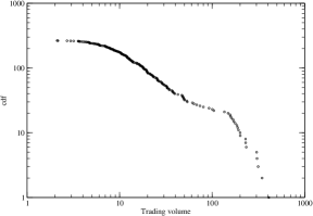
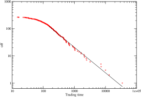
Figure 1: Cumulative distribution of average trading size (left) and waiting time in minutes (right) across banks.

In figure 1 we plot the cumulative distribution of average volumes (left) and average waiting times (right) across banks. The distribution of average waiting times is power law, revealing that there is not a typical scale for the trading frequency in the system.

In figure 2 we plot the distribution of waiting times, over the four year periods, for two highly active banks. We find that the distribution follows a stretched exponential of the form $a\exp(-t/\tau)^{\beta}$ [1]. The parameters of the fit for the two banks are reported in table 1.

We denote the signed trading volume as the cumulative volume of transactions for a single bank, where every transaction is added with a plus sign if the transaction is a sell, and with a minus sign if the transaction is a buy. As an example, if a bank starts with a given liquidity, lends some money and then borrows it to restore the initial liquidity, the total signed trading volume will be positive and increasing in the beginning, then decreasing to zero thereafter.

Bank code	$a$	$\tau$	$\beta$	$<dT>$ (minutes)
1	35589	5.90	0.466	16
70	10315	16.14	0.396	27

Table 1: Parameter estimation for the cumulative distribution function of waiting times for two highly active banks. The distribution is fitted to a stretched exponential of the form $a\exp(-t/\tau)^{\beta}$. $<dT>$ is the average waiting time between transactions for the two banks.

Hence we compute the signed trading volume $\bar{V}_{t}^{i}$, where the superscript $i$ denotes the bank, and we analyze their correlation matrix. Figure 3 shows the signed trading volume time series for a number of banks. It is apparent that there are some banks that follow correlated strategies and others that follow anticorrelated strategies. A structural break clearly appears in July 2001, when some banks inverted their trading behavior. This change of behavior can be associated with two events, at least. First, the official and market interest rates of the Euro area changed their trend from positive to negative at the beginning of 2001. Money market rates started increasingly to price in a reduction in the ECB interest rates of 25 basis points that was eventually decided on 30 August 2001. Furthermore the amount of liquidity provided by the European Central Bank increased in the summer 2001 to support economic growth.

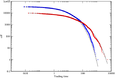
Figure 2: Distribution of waiting time for two banks and their corresponding stretched exponential fit. The parameters of the fit are reported in table 1.

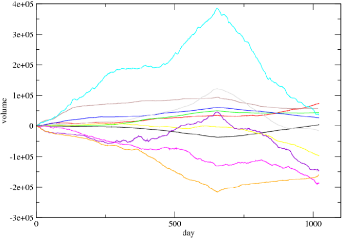
Figure 3: Sample of banks’ strategies.

There are many issues in computing the variance-covariance matrix. First, we do not observe changes of signed volume in continuous time, but only in form of discrete changes which occur when a transaction between two banks takes place. Second, the transactions do not occur at the same time. Thus, given two banks, the changes in signed volume are not synchronous. Furthermore some banks can trade more often than others and we observe a wide spectrum of trading frequencies. These difficulties make the implementation of a classical Pearson-like variance-covariance estimator problematic.

To circumvent these difficulties, we adopt the Fourier estimator of [2] instead. This is based on the following idea. Take a number of trajectories $X_{i}$ observed in $[0,2\pi]$, and compute the Fourier coefficients $a_{k}(dX_{i}),b_{k}(dX_{i})$ of $dX_{i}$. Then, the covariance between $X_{i}$ and $X_{j}$ is estimated via:

$$Cov(X_{i},X_{j})\simeq\frac{1}{M}\sum_{k=1}^{M}\left[a_{k}(dX_{i})a_{k}(dX_{j})+b_{k}(dX_{i})b_{k}(dX_{j})\right]$$ (1)

where $M$ is the largest frequency employed in computation which has to be suitably selected. The actual covariance is estimated in the limit $M\rightarrow\infty$. The methodology is model-free, and it produces very accurate, smooth estimates. Most importantly, it handles the time series in their original form without any need of imputation or data discarding. The estimator is based on integration of the time series to compute the Fourier coefficients, thus it is well suited to the uneven structure of the data. Moreover, it has a natural interpretation in the frequency domain, which is exactly what we aim to take care of, given banks’ different trading frequencies. This estimator has been shown to perform much better than the Pearson estimator in this kind of situations [3],[4]. It also performs well in estimating univariate volatility in the presence of microstructure noise[5]. Typically, it has been used for financial markets asset prices, e.g. on foreign exchange rates [6][7], stock prices [8] and stock index futures prices [9,10,11]. In this paper, we use it to analyze the cross-correlation among cumulative volumes. We refer to the quoted papers for the description of the implementation.

When computing covariances, we have to select carefully the maximum frequency employed in the computation. When the frequency increases we observe the Epps effect [12], that is the absolute value of the correlation is biased toward zero, see [3]. This is evident in Figure 4, where we show (left) the correlation as a function of the frequency for two given bank trading strategies, and (right) the average positive and negative correlation among all banks. It is important to remark that, given the definition of the trading strategy $\bar{V}_{i}$, whenever a bank increases its cumulative volume, there is a bank which decreases its cumulative volume, namely the bank who traded with it. Thus, negative correlations among trading strategies arise naturally. Since the less active bank in our sample makes about 1,000 transactions, we can choose a maximum cut-off frequency $M=500$, where $M$ is the largest Fourier harmonic used in (1). We compare two different frequencies, $M=100$, corresponding to a time scale of nearly $10$ days, and $M=500$, corresponding to a time scale of a couple of days. The largest the frequency the smallest the error and the largest the bias toward zero. Figure 5, shows the distribution of the correlations among trading strategies for $M=100$ and $M=500$. Correlations with $M=500$ are more centered around zero, because of the Epps effect, nonetheless there is not a great difference between the two, indicating that the bias is not so relevant. Thus the following results are obtained using $M=500$.

3 Principal Component Analysis

We analyze the correlation matrix of the trading strategies with the technique of random matrix theory (RMT), in line with the work of [13,14] on stock prices. Random matrix properties are derived in [15]. We find that at least two eigenvalues do not fit the predictions of RMT, see the inset in Figure 6. The economic interpretation of this fact is quite straightforward. If a bank lends and borrows over time in a non strategic way, the correlation among trading strategies should conform to the predictions of RMT. The fact that this is not the case means that banks do not behave randomly but a certain level of coordination can be observed. [16] for example have shown that over 2002 small banks have overall been acting as lenders, while larger banks have overall been acting as borrowers.

We finally check whether there is some deterministic pattern in the evolution of trading strategies over the maintenance period. To this purpose we compute the daily correlation matrices, and average those which are at the same distance from the EOM. It is well known that the behavior of banks is different near the EOM [16,17,18]

We find that the first eigenvalue has a decreasing explanatory power over the maintenance period, see Figure 7. On the contrary, the impact of the second largest eigenvalue, shown in the inset of figure 7, is constant over the maintenance period.

In the very first day of the maintenance period there is no distinct coordination among the strategies. Coordination increases and then it declines gradually in the last few days of the maintenance period. The interpretation of this empirical result is quite straightforward. When the EOM day is approaching, banks take more care in fulfilling their reserve obligations than in pursuing their preferred strategy (being a lender or a borrower). Thus, they transact more for pure liquidity reasons, and the correlation among trading strategies is less strong.

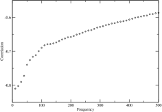
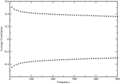
Figure 4: Epps effect in the correlations of two individual banks, bank 1 and bank47 (left) and average Epps effect (right).

Figure 5: Correlation distribution at two different cut-off frequencies.

Figure 6: Eigenvalues distribution at $M=500$ for the smallest eigenvalues (histogram) together with the prediction of RMT (dashed line). In the inset, the whole distribution is shown.

Figure 7: Explanatory power of largest eigenvalue as a function of the distance from EOM day. In the inset the same plot for the second largest eigenvalue

4 Communities structure

The aim of this section is to identify groups, or communities, of banks with similar trading strategies. To help visualizing the results we use the following taxonomy. We represent large Italian banks with blue circle, foreign banks with red circles, medium Italian banks with green and small banks with yellow. The two banks labeled in pink are two central institute of categories.

A simple way to identify communities in the system is to plot the correlation matrix as a graph, where banks are the vertices and links among them exist their strategies are positively correlated. Figure 8 (left) clearly evidences two separate communities of banks. To test that the two communities are not present only when selecting the frequency $M=500$ we have repeated the calculations by changing $M$. The results are consistent at all frequencies. For example in figure 9 (top) we plot the results obtained by selecting a lower frequency $M=25$, which correspond to a time scale of about one month and including all banks that trade at least once a month. Trading of bank reserves at different frequencies is driven in principle by different consideration. On an intra-day level, the main determinant is to target overnight balance without exceeding exposure limits, while on a monthly level, the aim is to meet reserve requirements. Movements in reserves at a lower frequency are mainly determined by the developments in banks’ other balance sheet positions over which banks have little control so that banks may not be able to play strategically at low frequencies but they may be acting strategically over longer time scales. Nonetheless we do not observe a clear difference in the correlation matrices over the two time scales and we still observe the same two communities in the correlation network in figure 9 (top).

To check that the method does not introduce spurious correlations and that communities do not emerge purely from the fact that the in the market there are simultaneously buyers and selles we have repeated the calculations of correlations by reshuffling the transactions (i.e. assigning each transaction to a random buyer and a random seller). The resulting graph is plotted in Figure 9 (bottom). In this case clearly no comunities emerge.

In figure 10 we plot the minimum spanning tree generated by the correlation matrix using the definition of distance given in [20,21]. On this tree, we can identify the same two communities identified before. The branches departing from bank number 103 are exactly the two groups on the left and the right of figure 8. In figure 11 we plot the overall correlation matrix where banks are ordered according to the hierarchical tree of figure 10, as in [22]. Again two distinct groups appear.

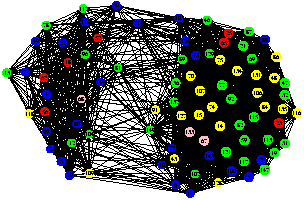
Figure 8: Positive correlation graph.

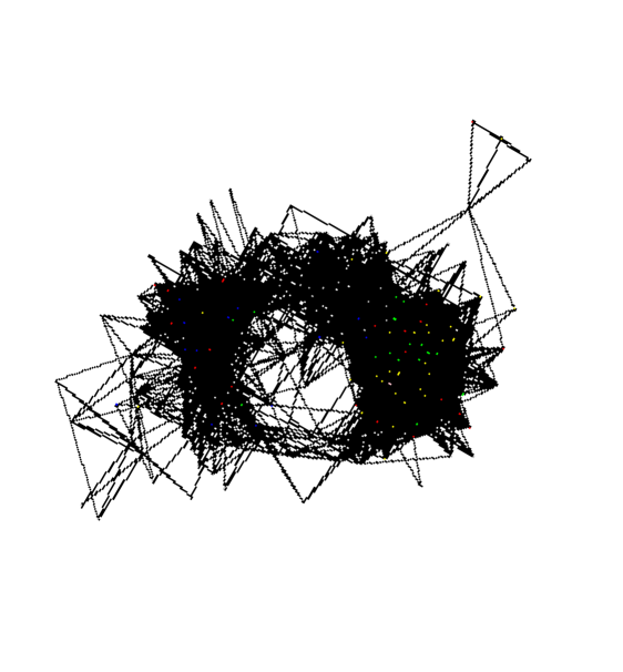
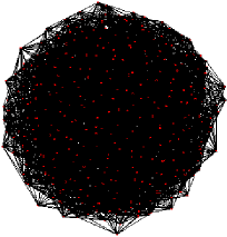
Figure 9: Positive correlations graph for all banks and M=25, for original transactions (top) and reshuffled transactions (bottom).

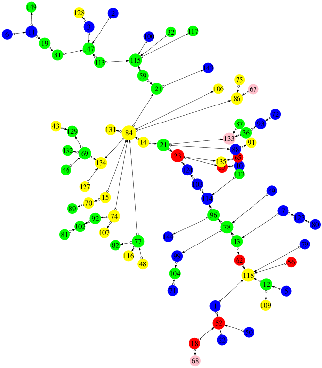
Figure 10: MST of correlations.

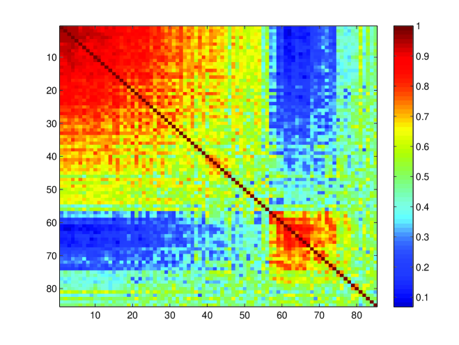
Figure 11: Correlation matrix. Banks are ordered according to the hierarchical tree of figure 10.

More sophisticated techniques for detecting community structure have been proposed in the last few years [23,24,25,26,27,28]. Some of them are based on the edge betweenness introduced by [29], also known as the NG–algorithm. To detect communities with this method the algorithm removes the edges with largest betweenness and in doing so it splits, step by step, the whole network into disconnected components. One problem with this method is that there is not an established criterion to stop the splitting process unless one knows, a priori, how many communities there are. To overcome such problems, approaches based on the spectral analysis have been recently adopted [30]. This approach does not need any a priori knowledge about the number of communities in the network (which is the most common case in actual networks) but it is based on a constrained optimization problem, in which we consider the nodes of the networks as objects linked by an harmonic potential energy.

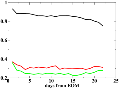
Figure 12: Distance from value 1 of the second, third and fourth eigenvalues for all days of the month: only the second eigenvalue is close to one indicating that only two communities are present. The second eigenvalue is closer to one on the EOM indicating that communities become more pronounced.

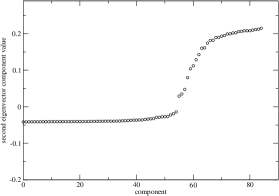
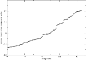
Figure 13: (Left) Second eigenvector components: the presence of a step like profile reveals the presence of two communities in the network. (Right) Second eigenvector components for the reshuffled matrix.

Detected	First	Second
communties	Community	Community
	113, 147, 115,	114, 112, 81, 52,
	23, 121, 21, 84,	96, 91, 109, 80,
	59, 82, 135, 2,	22, 49, 78, 123,
	86, 106, 47, 15,	79, 56, 12, 7,
	32, 134, 14, 107,	13, 118, 62, 1
	143, 131, 74, 67,
	100, 3, 116, 88,
	31, 87, 70, 92,
	77, 10, 133, 48,
	89, 71, 19, 36,
	128, 117, 50, 129,
	149, 69, 6, 127,
	124, 75, 102, 25,
	18, 46, 132, 103

Table 2: Communities detected

Many spectral methods [31,32,33] are based on the analysis of simple functions of the (weighted) connectivity matrix $A$, identified here as the correlation matrix. In particular, the functions of $A$ adopted are the Laplacian matrix $L=K-A$ and the Normal matrix $N=K^{-1}A$, where $K$ is the diagonal matrix with elements $k_{ii}=\sum_{j=1}^{n}a_{ij}$ and $n$ is the number of nodes in the network. In most approaches, concerning undirected networks, $A$ is assumed to be symmetric. The matrix $N$ has always the largest eigenvalue equal to one, due to row normalization. In a network with an apparent cluster structure, the matrix $N$ has also a certain number $m-1$ of eigenvalues close to one, where $m$ is the number of well defined communities, the remaining eigenvalues lying a gap away from one. The eigenvectors associated to these first $m-1$ nontrivial eigenvalues, also have a characteristic structure. Define $x_{i}$ as the position if the $i$-th vertex after sorting vertices by the value of its corresponding component in one eigenvector. The components corresponding to nodes within the same cluster have very similar values $x_{i}$, so that, as long as the partition is sufficiently sharp, the profile of each eigenvector, sorted by components, is step-like. The number of steps in the profile gives again the number $m$ of communities. Here we find just one eigenvalue close to one (see figure 12), suggesting the existence of only two communities. We analyze the component of the associated second eigenvector in the left side of figure 13 which shows the characteristic step like profile, identifying the two communities. As shown in Table 2 the communities are the same as those in figure 8. The group on the top right in figure 13 corresponds to the group on the left in figure 8. On the right side of figure 13 we plot the second eigenvector components for the correlation matrix obtained by reshuffling the transactions. The step like shape is not visible in this case.

As the second eigenvalue approaches one, the communities becomes better defined. Figure 12 shows that near the EOM communities become more pronounced. This is not in contrast with our previous finding that the overall level of aggregation in the system decreases when EOM approaches. In fact, the overall correlation may decrease while the correlation of strategies inside the same community can become stronger. The separation between the two communities is less pronounced far from the EOM. We have also observed that very few banks change community during the maintenance period.

Finally we note that the first community is composed predominantly of large and foreign banks (red and blue circles if figure 8) while the second community involves predominantly small banks (green and yellow circles if figure 8). Furthermore, the first community displays a pronounced geographical feature, that is all banks belonging to it are located in the northern part of Italy.

5 Conclusions

We investigated the Italian segment of the European money market over the period 1999-2002 using a unique data-set from which it is possible to reconstruct the trading strategy of each participating bank. We used the Fourier method to estimate the variance-covariance matrix that we analyzed, since it is the most suitable to the unevenly structure of the data. We then analyzed the variance-covariance matrix using standard PCA and tools borrowed from the analysis of complex networks. We find that two main communities emerge, one mainly composed by large and foreign banks, the other composed by small banks. Banks act predominantly as borrowers or lenders respectively, with an inversion of their behavior in July 2001. Moreover, the analysis reveals that while overall trading strategies becomes less correlated when the EOM approach, the communities become more pronounced on the EOM date.

Aknowledgements

We thankfully acknowledge financial support from the ESF–Cost Action P10 ”Physics of Risk”.

References

[1] E. Scalas, R.Gorenflo, H.Luckock, F.Mainardi, M.Mantelli, and M.Raberto, Quantiative Finance 4 (6) (2004) , 695-702.

[2] P. Malliavin and M. Mancino, Finance and Stochastics, 6 (1) (2002), 49-61.

[3] R. Reno’, International Journal of Theoretical and Applied Finance, 6 (1) (2003), 87-102.

[4] O. Precup, G. Iori, Physica A 344 (2004), 252–256.

[5] M.O. Nielsen and P.H. Frederiksen, Working paper, Cornell University. (2005).

[6] E. Barucci and R.Reno’, Journal of International Financial Markets, Institutions and Money 12 (2002), 183-200

[7] E. Barucci and R.Reno’, Economics Letters 74(2002), 371-378.

[8] M. Mancino and R. Reno’, Applied Mathematical Finance 12 (2) (2005), 187-199.

[9] R. Reno’ and R. Rizza, Physica A 322 (2003), 620-628.

[10] M. Pasquale and R. Reno’, Physica A 346 (2005), 518-528.

[11] S. Bianco and R. Reno’, Journal of Futures Markets 26 (1) (2006), 61-84.

[12] T. Epps, Journal of the American Statistical Association 74 (1979),291-298.

[13] V. Plerou, P.Gopikrishnan, B.Rosenow, L.NunesAmaral, and E.Stanley, Physical Review Letters 83(7)(1999), 1471-1474.

[14] L. Laloux, P.Cizeau, J.-P. Bouchaud, and M.Potters , Physical Review Letters 83 (7) (1999), 1467-1470.

[15] Mehta, M., ”Random matrices”, Academic Press, New York (1995).

[16] G. Iori, G.DeMasi, O.Precup, G.Gabbi, and G.Caldarelli, A network analysis of the Italian interbank money market, submitted paper (2005).

[17] P.Angelini, Journal of Money, Credit and Banking 32, (2000) 54-73.

[18] E. Barucci, C.Impenna, and R.Reno’, The Italian overnight market: microstructure effects, the martingale hyphotesis and the payment system, Temi di Discussione, Bank of Italy N. 475 (2003).

[19] T. Kamada and S.Kawai, An algorithm for drawing general inderected graphs, Information Processing Letters 31 (1) (1989), 7-15.

[20] R.N. Mantegna, and H.E. Stanley, An introduction to econophysics, Cambridge University Press (2000)

[21] G. Bonanno, F.Lillo, and R.N. Mantegna, Quantitative Finance 1 (2001), 1-9.

[22] G. Bonanno, F.Lillo, and R.N. Mantegna, Physica A 299 (2001), 16-27.

[23] F. Radicchi, C.Castellano, F.Cecconi, V.Loreto, and D.Parisi, Proceedings of the National Academy of Science of USA, 101(9) (2004), 2658-2663.

[24] J. Reichardt and S. Bornholdt Physical Review Letters 92 (21) (2004), 218701.

[25] A. Clauset, M.E.J. Newman, and C.Moore, Physical Review E 70 (2004), 066111.

[26] M. E.J. Newman, SIAM Review 45 (2) (2003), 167-256.

[27] J. Duch and A.Arenas, Physical Review E 72 (2005), 027104.

[28] L. Danon, A.Diaz-Guilera, J.Duch, and A.Arenas, Journal of Statistical Mechanics, P09008 (2005).

[29] M. Girvan, and M.E.J. Newman, Proceedings of the National Academy od Science of USA 99 (12) (2002), 7821.

[30] A. Capocci., V.D.P. Servedio, G.Caldarelli, and F.Colaiori, Physica A 352 (2-4) (2005), 669-676.

[31] K.M. Hall, Management Science 17(1970), 219.

[32] A.J. Seary and W. D. Richard, Proceedings of the International Conference on Social Networks, 1: Methodology, Volume 47 (2005).

[33] J.M. Kleinberg, ACM Computing surveys 31(4es), 5 (1999).