Bending Wavelet for Flexural Impulse Response

Abstract

The work addresses the definition of a wavelet that is adapted to analyse a flexural impulse response. The wavelet gives the opportunity to directly analyse the dispersion characteristics of a pulse. The aim is to localize a source or to measure material parameters. An overview of the mathematical properties of the wavelet is presented. An algorithm to extract the dispersion characteristics with the use of genetic algorithms is outlined. The application of the wavelet is shown in an example and experiment.

1 Introduction

The Morlet wavelet transform is a popular method for time-frequency analysis. Its application for acoustic signals can be found in several publications. These publications deal for example with the analysis of dispersive waves onsay ; kishimoto , source or damage localization yamada ; gaulident ; rucka ; junsheng ; railroad ; messina , investigation of system parameters hayashi ; ta or active control berry98wavelet . A comparison of the short time Fourier transform and the Morlet wavelet transform is done by Kim et.al. kimkim . It is found that the continuous wavelet transform CWT of acoustic signals is a promising method to obtain the time - frequency energy distribution of a signal.
These applications are based on the evaluation of the frequency dependent arrival time of a pulse in dispersive media. The underlying concept of this method will be briefly explained for a one-dimensional structure (e.g. a beam).
A fundamental difference between most waveforms in structures and fluids is the dispersion. A pulse propagating in a structure with the frequency dependent group velocity $c_{g}$ changes its shape. Due to this dispersion the pulse is not recognizable with correlation techniques that can be useful for locating airborne sound sources micarray .
The wavelet transform is very useful to extract exactly the arrival time $t_{a}$ of an pulse in a dispersive media

$$t_{a}=x/c_{g}.$$ (1)

The continuous wavelet transform $W_{\psi}^{y}$ of a function $y$ is

$$W_{\psi}^{y}(a,b)=\frac{1}{\sqrt{c_{\psi}|a|}}\int\limits_{-\infty}^{\infty}y(t)\>\psi\left(\frac{t-b}{a}\right)\>dt.$$ (2)

The analogue to the Fourier transforms spectrogram is the scalogram defined as $|W_{\psi}^{y}(a,b)|^{2}$. It can be shown that for a fixed scaling parameter $a$ the arrival time $t_{a}$ is the point in time where the maximum of the scalogram occurs

$$max\left(|W_{\psi}^{y}(a,b)|^{2}\right)=|W_{\psi}^{y}(a,b=t_{a})|^{2}.$$ (3)

To locate a source one needs

1. the point in time the pulse occurred, the group velocity and a sensor, or

2. two sensors, or

3. one sensor measuring two distinguishable wave types jiao .

If the position of the source is known, it is possible to extract material parameters hayashi ; ta .
To improve this method, dispersion based transforms have been proposed yoonkim ; liu , which is based on a method called Chirplet transform mannVI91 ; mannsp . These transforms improved the analysis. Nevertheless the bending wavelet that is presented is a new approach.
Here a different wavelet suitable for bending waves which can be modelled with the Euler beam theory is presented.
The underlying concept is not to measure the arrival time but to extract directly the dispersion of the pulse. The dispersion of the pulse is dependent on the distance between source and receiver and the material properties. If it is possible to extract exactly the spreading of the pulse one has directly the distance or the material properties, depending on which is known. To define a wavelet that extracts the dispersion characteristics it is necessary to know the impulse response function in the time domain. For plates which can be modelled with the Euler beam theory this function is derived first by Boussinesqboussinesq and can be found in textbooksheckl . For beams it is treated in a companion publicationbendimpulse since only the Green’s functions for a initial deflection and velocity are found in the literaturenowacki ; meirovitch .
The velocity $v(r,t)$ resulting from the bending wave propagation on a infinite plate of a force impulse $F_{a}(t)=F_{0}\>\delta(t)$ at $r=0$ is

$$v(r,t)=\frac{\hat{F}_{0}}{4\pi t\sqrt{B^{\prime}m^{\prime\prime}}}\sin\left(\frac{r^{2}}{4\zeta t}\right),$$ (4)

where $r$ is the distance from the source, $\zeta=\sqrt{B^{\prime}/m^{\prime\prime}}$, bending stiffness $B^{\prime}=Eh^{3}/(12(1-\nu^{2}))$, $E$ the elastic or Young’s modulus, $h$ the plate thickness, $\nu$ the Poisson’s ratio and $m^{\prime\prime}$ the mass per unit area.
The bending wave velocity $v(x,t)$ on a infinite beam, resulting of a force impulse $F_{a}(t)=F_{0}\>\delta(t)$ at $x=0$ is given by

$$v(x,t)=\frac{F_{0}H(t)}{m^{\prime}}\sqrt{\frac{2}{\pi\zeta t}}\cos\left(\frac{x^{2}}{4\zeta t}\right)\>.$$ (5)

therein $x$ is the distance from the source, $\zeta=\sqrt{B/m^{\prime}}$, where $B$ is the bending stiffness of the beam and $m^{\prime}$ mass per unit length.
The term

$$d_{i}=\frac{x^{2}}{4\zeta}.$$ (6)

is the factor that controls this spreading and is called dispersion factor. Whereas the dispersion factor is a time value the nondimensional term

$$Di=\frac{x^{2}f_{max}}{4\zeta},$$ (7)

is called dispersion number. The applicability of the following method depends on the dispersion number. Higher dispersion numbers result in a longer useful time period and this case is better to analyse. An exact quantification is given in the following, equation (25). A high dispersion number is the reason for choosing a thin plate and a slender beam.
In the following a new adapted wavelet will be derived to extract the dispersion factor from the measured pulse. Usually a wavelet is designed to localize a certain frequency. In contrary the proposed wavelet localizes a frequency range that is distributed over the wavelet length just like equation (4) or (5). Such a choice follows the paradigm of signal processing, that ”the analysing function should look like the signal”.
One may interpret the continuous Wavelet transform as a cross-correlation of $y$ and $\psi$. Hence, the idea is to find the function which is highly correlated with the impulse response. The difference is the role of the scaling parameter $a$. It is vital to produce the presented results to use the scaling parameter as it is defined in equation (2).
The dispersion factor is determined by the scaling factor with the highest value of the scalogram. In principle this can be done with a fine grid of $(a,b)$ values. A more efficient way is to use an optimisation scheme. Gradient based optimisation is not reliable in finding a global optimum. A second problem is the localisation of several overlapping pulses. A well known method that is able to fulfill these requirements are genetic algorithms.

2 Bending wavelet

Several different definitions based on the Morlet wavelet and the Chirplet transformmannVI91 ; mannsp have been investigated. For brevity an extensive discussion about the different efforts is omitted. The details of the mathematical background of the wavelet transform can be found in the literature Mallat98wavelet ; wavelets .
The section begins with the definition of a wavelet with compact support and zero-mean. It follows a comment on the amplitude and frequency distribution and ends with possible optional definitions.

2.1 Definition

The mother wavelet

$$\psi_{s}(t)=\left\{\begin{array}[]{ll}\frac{\sin(1/t)}{t}&\mbox{ for }t_{min}<t<t_{max}\\ 0&\mbox{ otherwise}\end{array}\right.,$$ (8)

is called bending wavelet.
A wavelet $\psi$ must fulfill the admissibility condition

$$0<c_{\psi}=2\pi\int\limits_{-\infty}^{\infty}\frac{|\hat{\psi}(\omega)|^{2}}{|\omega|}\>d\omega<\infty,$$ (9)

where $\hat{\psi}(\omega)$ is the Fourier transform of the wavelet. The proposed wavelet (8) has a compact support $(t_{min},t_{max})$, which means that the admissibility condition is fulfilled if

$$\int\limits_{t_{min}}^{t_{max}}\psi(t)\>dt=0$$ (10)

holds. To fulfill the admissibility condition $t_{min}$ and $t_{max}$ are defined so, that equation (10) holds. With the integral - sine function $\mbox{Si}(x)=\int_{0}^{x}\sin(t)/t\>dt$ one finds that

$$\int\limits_{t_{min}}^{t_{max}}\frac{\sin(1/t)}{t}\>dt=\mbox{Si}\left(\frac{1}{t_{max}}\right)-\mbox{Si}\left(\frac{1}{t_{min}}\right).$$ (11)

Since $\lim_{t\to 0}\mbox{Si}(1/t)=\pi/2$ and that the Si-function for $t<2/\pi$ oscillates around $\pi/2$, one is able to chose $t_{min}$ and $t_{max}$ so, that

$$\mbox{Si}(1/t_{min})=\mbox{Si}(1/t_{max})=\pi/2.$$ (12)

This is a very easy option to define a wavelet and it will be used later to define similar wavelets. Equation (12) can only be solved numerically so a good approximation should be used that leads to a simple expression for $c_{\psi}$. The support of the wavelet is defined by

$$\frac{1}{t_{min/max}}=\frac{(2n_{max/min}-1)\pi}{2}.$$ (13)

The function $\mbox{Si}(1/t)$ and proposed possible values of $t_{min}$ or $t_{max}$ are plotted in figure 1. In the worst case for $t_{max}=2/\pi$ and $t_{min}\rightarrow\infty$ the difference in equation (10) is around $0.2$, but for higher values of $n_{min}$ the magnitude is in the order of other inaccuracies, so that it should be negligible. Like the Morlet wavelet, which fulfills the admissibility condition in a asymptotic sense the bending wavelet fulfills the admissibility for $\lim t\rightarrow 0$.

Figure 1: $\mbox{Si}(1/t)$ and circles at $1/t=(2n-1)\pi/2$

The value of the constant is calculated $c_{\psi}$ with the norm in the Lebesque space $L^{2}$ of square integrable functions

$$||\psi(t)||_{2}=\left(\int\limits_{-\infty}^{\infty}\psi(t)^{2}\>dt\right)^{1/2}.$$ (14)

The integral in equation (14) is

$$\begin{array}[]{l}\int\limits_{t_{min}}^{t_{max}}\sin(1/t)^{2}/t^{2}\>dt=\\ \frac{1}{4}\left(\frac{2}{t_{min}}-\frac{2}{t_{max}}-\sin\left(\frac{2}{t_{min}}\right)+\sin\left(\frac{2}{t_{max}}\right)\right).\end{array}$$ (15)

With the proposed choice of $t_{min}$ and $t_{max}$, the sine vanishes and a normalised $||\psi(t)||_{2}=1$ wavelet is obtained if $c_{\psi}$ is chosen to be

$$c_{\psi}=\frac{1}{2}\left(\frac{1}{t_{min}}-\frac{1}{t_{max}}\right)=\frac{\pi}{2}(n_{max}-n_{min}).$$ (16)

2.2 Displacement-invariant definition

Wavelets that are defined by real functions have the property that the scalogram depends on the phase of the analysed function. Wavelets that are complex functions like e.g. the Morlet wavelet are called displacement-invariant. A wavelet $\psi=\psi_{c}+i\psi_{s}$ that consists of a sine, $\psi_{s}$ equation (8), and a cosine wavelet which is

$$\psi_{c}(t)=\left\{\begin{array}[]{ll}\frac{\cos(1/t)}{t}&\mbox{ for }t_{min}<t<t_{max}\\ 0&\mbox{ otherwise}\end{array}\right..$$ (17)

can be beneficial. With the integral - cosine function $\mbox{Ci}(x)=\int_{0}^{x}\cos(t)/t\>dt$ one finds that

$$\int\limits_{t_{min}}^{t_{max}}\frac{\cos(1/t)}{t}\>dt=\mbox{Ci}\left(\frac{1}{t_{max}}\right)-\mbox{Ci}\left(\frac{1}{t_{min}}\right).$$ (18)

The analogous definition of the value $\pi/2$ for the Ci-function is

$$\mbox{Ci}(1/t_{min})=\mbox{Ci}(1/t_{max})=0.$$ (19)

The approximation is given by

$$\frac{1}{t_{min/max}}=n_{max/min}\pi.$$ (20)

The effect is that the real- and the imaginary part of the resulting wavelet do not share the same support. This is an awkward definition of a mother wavelet but the difference between the two supports is rather small if the same value for $n_{max/min}$ is used. To keep things simple only the real valued sine wavelet is used in following.

2.3 Orthogonality of the bending wavelet

The trigonometric functions that are used for the Fourier transform establish an orthogonal base. Hence, the Fourier transform has the convenient characteristic that only one value represents one frequency in the analysed signal. Every deviation of this is due to the windowing function that is analysed with the signal. Already the short time Fourier transform is not orthogonal, if the different windows overlap each other. Because of this overlap the continuous wavelet transform can not be orthogonal. The proposed wavelet should still be investigated since it is instructive for the interpretation of the results.
The condition for an orthogonal basis in Lebesgue space $L^{2}$ of square integrable functions is

$$(\psi_{j},\psi_{k})=\int\limits_{-\infty}^{\infty}\psi_{j}\psi_{k}=\delta_{jk}.$$ (21)

Two different wavelets $\psi_{j}$ and $\psi_{k}$ can be obtained by using different scaling parameters $a$ and/or different displacement parameters $b$. Here the effect of two scaling parameters is investigated, so the following integral is to be solved

$$\int\limits_{-\infty}^{\infty}a_{j}a_{k}\sin(a_{j}/t)\sin(a_{k}/t)/t^{2}\>dt.$$ (22)

To illustrate the integral, two different versions of the wavelet are plotted in figure 2.

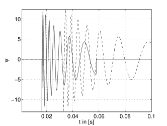
Figure 2: Bending wavelet (8) for $a_{1}=1$ (solid) and $a_{2}=2$ (dashed), $n_{min}=4$ and $n_{max}=12$

One finds that

$$\begin{array}[]{l}\int\limits_{-\infty}^{\infty}a_{j}a_{k}\sin(a_{j}/t)\sin(a_{k}/t)/t^{2}\>dt=\\ \left.\frac{a_{j}a_{k}}{a_{k}^{2}-a_{j}^{2}}\left(a_{j}\cos\left(\frac{a_{j}}{t}\right)\sin\left(\frac{a_{k}}{t}\right)-a_{k}\cos\left(\frac{a_{k}}{t}\right)\sin\left(\frac{a_{j}}{t}\right)\,\right)\right|_{t_{min}}^{t_{max}}.\end{array}$$ (23)

The sine term in equation (23) vanishes since $t_{min/max}$, also scale with $a$, but actually there are two different values of $a$ and so not all four sine terms vanish. With this result one expects a rather broad area in $(a,b)$ with high values of the scalogram.

2.4 Time amplitude/frequency distribution

The time frequency distribution of the wavelet for a certain scaling factor $a$ is determined by the argument of the sine function. The instaneous frequency $\omega(t)$ can theoretical be obtained with a relationship for almost periodic functions, see Bochner bochnerfp . The actual frequency of the wavelet is given by

$$\sin\varphi(t)\rightarrow\omega(t)=\varphi^{\prime}(t)=\frac{a}{t^{2}}.$$ (24)

The $1/t$ leading term affects the amplitude of the wavelet. Usually it is desired that the whole signal contributes linearly to the transform. To achieve this it is useful to have an amplitude distribution over time of the wavelet that is reciprocal to the amplitude distribution of the analysed signal. Since the bending wavelet has the same amplitude distribution as equation (4) this may lead to stronger weighting of the early high frequency components of the impulse response.
A force impulse that compensates the amplitude distribution of the impulse response follows a $\sim 1/\omega^{2}$ dependence.

3 Continuous wavelet transform with the bending wavelet

The application in the given context is to extract precisely the scaling factor with the highest value. How this is achieved will be discussed in the next section. Here the realisation of a transform with a set of scaling factors is presented since it is illustrative.
The algorithm implementing the continuous wavelet transform with the bending wavelet can not be the same as the algorithm implementing a transform with any continuous wavelet, like the Morlet wavelet. The bending wavelet has a compact support, which must be defined prior to the transform. This can be done with a estimation of the frequency range and the dispersion number. With the equations (13) and (24) it holds that

$$n_{max} = \mbox{floor}\left(\sqrt{\frac{d_{i}f_{max}}{2\pi}}+\frac{1}{2}\right)$$

$$n_{min} = \mbox{ceil}\left(\sqrt{\frac{d_{i}f_{min}}{2\pi}}+\frac{1}{2}\right),$$ (25)

where floor$(\cdot)$ rounds down towards the nearest integer and ceil$(\cdot)$ rounds up. The knowledge of a useful frequency range should not provide any problems. But to have to know beforehand which dispersion number will dominate the result is rather unsatisfactory. A more practical solution is to calculate the corresponding $n$-value within the algorithm, which is an easy task since $a=d_{i}$. The problem with this possibility is that the support of the wavelet changes within the transform. Since the support is part of the wavelet this means that strictly one compares the results of two different wavelets. Since the wavelet is normalised the effect is rather small, but nevertheless it should be interpreted with care.

3.1 Example

To illustrate the use of the proposed wavelet the following function is transformed

$$y(t)=\left\{\begin{array}[]{ll}t\sin(a/t),&\mbox{ for }t_{min}<t<t_{max}\\ 0&\mbox{otherwise,}\end{array}\right.$$ (26)

with $a=10$. The sampling frequency is $f_{s}=2^{9}$, $t_{min}$ and $t_{max}$ are defined by the corresponding values of $f_{max}=f_{s}/8$ and $f_{min}=4$, for convenience the point $t=t_{min}$ is shifted to $10\Delta t$. The example function in equation (26) is plotted in figure 3.

Figure 3: Analysed example function (26)

The example function is transformed with the algorithm that calculates $n_{min}$ and $n_{max}$ with the corresponding value of $f_{max}$, $f_{min}$ and $a$. The choice of the frequency range is critical. If it is too small, information will be lost and if it is too big the parts that overlap the pulse may distort the result. Here the same frequency range as the analysed function is used.
The resulting scalogram is not plotted directly against the factor $b$, but shifted with the value of $t_{min}$. This means that the maximum value is at $10\Delta t$ (figure 4), which is the value of $t$ where $f_{max}$ is located. The maximum value is shifted when $f_{max}=f_{s}/12$ is used, as can be seen in figure 5.

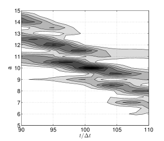
Figure 4: Contour plot of the scalogram build with the bending wavelet transform of equation (26) with $f_{max}=f_{s}/8$ and $f_{min}=4$

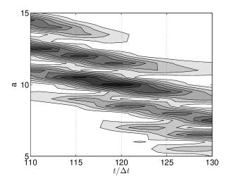
Figure 5: Contour plot of the scalogram build with the bending wavelet transform of equation (26) with $f_{max}=f_{s}/12$ and $f_{min}=4$

One may recognise that there are very high values if the wavelet is shifted and scaled along the curve $a/t$. This is expected theoretically, as discussed in section 2.3 and can be interpreted descriptive since the wavelet does not localize one frequency, but has a wide frequency range that spreads over time. It can be quantified with equation (21). Evaluating this integral numerically for the values of $a_{1}=10$, $a_{2}=11.75$ and $b_{2}=7\Delta t$ results in value of $0.68$, which means that the peak at $a_{2}=11.75$ has $68\%$ of the peak at $a_{1}=10$.
This problem of non-orthogonality is addressed by the following algorithm. The pulse is extracted from the signal by first locating the position $t_{start}$ in the signal, where $f_{max}$ has its maximum. This is done by a Morlet wavelet transform with which one may find the value of $t_{start}$ that has the highest value of $f_{max}$. Now the transformation with the bending wavelet is only done in the vicinity of $t_{start}$. Technically the displacement parameters $b$ are defined with $t_{start}$.

4 Localization with a Genetic Algorithm

Genetic algorithms (GA) form a particular class of evolutionary algorithms that use techniques inspired by evolutionary biology such as inheritance, mutation, selection, and crossover. Genetic algorithms are categorized as global search heuristics. Details of the method can be found in the extensive literature, e.g.pohlheim .
The genetic algorithm is chosen, since it is usually very reliable in finding a global optimum and its ability to find Pareto optimums to locate several pulses. However the drawback is the slow convergence, that can be improved with a local search method. Recent publications on this topic are gageo ; gacarin .
The implementation is done with functions provided by the open source Matlab toolbox gatoolbox , if not stated otherwise. Principally possible but not used in the example is the localization of two pulses that are overlapping. For the sake of brevity a discussion on how this can be achieved will be omitted. The algorithm works with two variables, the displacement parameter and the scaling factor of the bending wavelet.
The displacement parameter is defined by $t_{start}\pm\lambda/2$ or smaller values. This depends on the size of the Morlet wavelet. For discrete functions it is an integer value but nevertheless implemented as a floating point number, because of lacking support for such a combination in the toolbox. This fact is taken into account when calculating the wavelet transform. A pseudo-code that describes the genetic algorithm can be found in the appendix A.
In the end only the fittest individual is extracted. The algorithm is usually quite reliable. Since it is a stochastic method, it can be beneficial to restart the whole process or to work with several sub-populations.

4.1 Example

As an example, the already transformed equation (26) is investigated. The frequency range is the same as the example plotted in figure 5. As a first step the value $t_{start}$ is calculated with a Morlet wavelet transform at $f_{s}/12$. The result is plotted in figure 6, where the maximum is at $t_{i}=122$. From figure 5 one may conclude that the correct value is $120$ this slight deviation is due to the fact that the Morlet wavelet has a rather broad frequency resolution and the amplitude of the signal is increasing with time. If the signal $\sin(a/t)/t$ is used, the maximum is located at $118$. The number of individuals is chosen to $100$ and the number of generations to $400$.
The initial chromosome has a time index range of $(106,138)$ which is $3/4\lambda$ and the range of the scaling factor is $(5,15)$. The obtained scaling factor is $a=9.99$. The frequency range of the bending wavelet is shorter than the values $f_{wmax}=37.7<42.7=f_{s}/12$ and $f_{wmin}=4.756<4<f_{min}$, this due to equation 25. The wavelet with the best scaling factor and the example function are plotted together in figure 7. One may recognize that the frequency-time distribution of both function match.

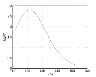
Figure 6: Morlet wavelet transform of equation (26) with $f=f_{s}/12$

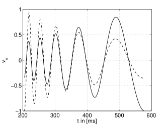
Figure 7: Bending wavelet at $a=9.99$ and the example function

4.2 Experimental results

Experiments on a beam and a plate are discussed in detail in combination with the impulse response functionsbendimpulse . The method was used to extract the dispersion factor $d_{i}$. The theoretical functions (4) and (5) with the obtained dispersion factor $d_{i}$ are compared with the measured curves. A good agreement of theory and experiment shows the applicability of the presented transform.

4.3 Comparision with Morlet Wavelet

The drawback of the proposed method is that it is only applicable to bending waves that can be modelled with the simple Euler beam theory or any wave that has a dispersion relation that follows a $\sim 1/\sqrt{\omega}$ dependence. Another precondition is the rather high dispersion number. Nevertheless bending waves are dominant in structure borne sound problems and for thin structures the simplifications of the Euler bending theory are usually valid.
The method is accurate, fast and easy to implement. In the experiments a source could be localized with a deviation lower than $10\%$. One can build real time applications for source detection. The method has also principle advantages, it is possible to

1. obtain the distance of a impulse or the material properties with only one measurement,

2. analyse two overlapping pulse, which is not possible with the maximum of the Morlet wavelet transform where for each frequency one maximum value is extracted.

5 Concluding Remarks

A definition of a new adapted wavelet, the bending wavelet, is given. The mathematical properties of the bending wavelet are discussed. It is shown in examples that the transform is useful to analyse a flexural impulse response.
Besides source localisation a possible application is the measurement of material properties in a built-in situation of finite structures, since the method does not depend on the boundary conditions.
The choice of a useful frequency range can be problematic. It may be useful to first analyse the signal with a Morlet wavelet transform to find a useful range.

Appendix A Appendix

1 Linear distributed
  initial chromosome of t and a.
2 Bending wavelet transform with
  the initial chromosome.
3 Assignment to the
  current population.
Repeat
    4 Self-written rank based
      fitness assignment (current pop.).
    5 Selection with
      stochastic universal sampling.
    6 Recombination with the
      extended intermediate function.
    7 Real-value mutation with
      breeder genetic algorithm.
    8 Bending wavelet transform with the
      selected chromosome.
    9 Self-written fitness based insertion
      with 70% new individuals.
Until max number of generations

References

- (1) T. Önsay, A. G. Haddow, Wavelet transform analysis of transient wave propagation in a dispersive medium, Acoustical Society of America Journal 95 (1994) 1441–1449.
- (2) K. Kishimoto, M. H. H. Inoue, T. Shibuya, Time frequency analysis of dispersive waves by means of wavelet transform, Journal of Applied Mechanics 62 (1995) 841–46.
- (3) H. Yamada, Y. Mizutani, H. Nishino, M. Takemoto, K. Ono, Lamb wave source location of impact on anisotropic plates, Journal of Acoustic Emission 18 (2000) 51–60.
- (4) L. Gaul, S. Hurlebaus, Identification of the impact location on a plate using wavelets, Mechanical Systems and Signal Processing 12 (6) (1998) 783–795.
- (5) M. Rucka, K. Wilde, Application of continuous wavelet transform in vibration based damage detection method for beams and plates, Journal of Sound and Vibration 297 (2006) 536–550.
- (6) C. Junsheng, Y. Dejie, Y. Yu, Application of an impulse response wavelet to fault diagnosis of rolling bearings, Mechanical Systems and Signal Processing 21 (2005) 920–929.
- (7) F. L. di Scalea, J. McNamara, Measuring high-frequency wave propagation in railroad tracks by joint time-frequency analysis, Journal of Sound and Vibration 273 (3) (2004) 637–651.
- (8) A. Messina, Detecting damage in beams through digital differentiator filters and continuous wavelet transforms, Journal of Sound and Vibration 272 (1) (2004) 385–412.
- (9) Y. Hayashi, S. Ogawa, H. Cho, M. Takemoto, Non-contact estimation of thickness and elastic properties of metallic foils by the wavelet transform of laser-generated lamb waves, NDT & E international 32/1 (1998) 21–27.
- (10) M.-N. Ta, J. Lardies, Identification of weak nonlinearities on damping and stiffness by the continuous wavelet transform, Journal of Sound and Vibration 293 (1) (2006) 16–37.
- (11) P. Masson, A. Berry, P. Micheau, A wavelet approach for the active structural acoustic control, Journal of the Acoustical Society of America 104 (3) (1998) 1453–1466.
- (12) Y. Kim, E. Kim, Effectiveness of the continuous wavelet transform in the analysis of some dispersive elastic waves, Journal of the Acoustical Society of America 110 (1) (2001) 86–94.
- (13) M. Brandstein, D. Ward, Microphone Arrays—Signal Processing Techniques and Applications, Springer, 2001.
- (14) J. Jiao, C. He, B. Wu, R. Fei, Application of wavelet transform on modal acoustic emission source location in thin plates with one sensor, International Journal of Pressure Vessels and Piping 81 (2004) 427–431.
- (15) J. C. Hong, K. H. Sun, Y. Y. Kim, Dispersion-based short-time fourier transform applied to dispersive waves, Journal of the Acoustical Society of America 117 (5) (2005) 2949–2960.
- (16) B. Liu, Adaptive harmonic wavelet transform with applications in vibration analysis, Journal of Sound and Vibration 262 (1) (2003) 45–64.
- (17) S. Mann, S. Haykin, The chirplet transform: A generalization of Gabor’s logon transform, Vision Interface ’91 (1991) 205–212.
- (18) S. Mann, S. Haykin, The chirplet transform: Physical considerations, IEEE Trans. Signal Processing 43 (11) (1995) 2745–2761.
- (19) J. Boussinesq, Application des potentials a l’etude de l’equilibre et du mouvement des solides elastiques, Gauthier-Villars, Paris, 1885.
- (20) L. Cremer, M. Heckl, B. Petersson, Structure-Borne Sound, Springer Verlag, 2005.
-
(21)
R. Büssow, Applications of the flexural impulse response functions in the
time domain, Acta Acoustica United with Acoustica (submitted) (2007).
URL http://arxiv.org/abs/physics/0610163/ - (22) W. Nowacki, Dynamics of Elastic Systems, Chapman and Hall LTD., 1963.
- (23) L. Meirovitch, Analytical Methods in Vibrations, Collier-Macmillan, 1967.
- (24) S. Mallat, A wavelet tour of signal processing, Academic Press, 1998.
- (25) A. Louis, P. Maaß, A. Rieder, Wavelets, B.G. Teubner, 1994.
-
(26)
S. Bochner, Beiträge zur Theorie der fastperiodischen Funktionen,
Mathematische Annalen 96 (1) (1927) 119–147. - (27) H. Pohlheim, Evolutionäre Algorithmen, Springer, 2000.
- (28) C. Park, W. Seong, P. Gerstoft, Geoacoustic inversion in time domain using ship of opportunity noise recorded on a horizontal towed array, Journal of the Acoustical Society of America 117 (4) (2005) 1933–1941.
- (29) L. Carin, H. Liu, T. Yoder, L. Couchman, B. Houston, J. Bucaro, Wideband time-reversal imaging of an elastic target in an acoustic waveguide, Journal of the Acoustical Society of America 115 (1) (2004) 259–268.
- (30) A. Chipperfield, P. Fleming, H. Pohlheim, C. Fonseca, The Genetic Algorithm Toolbox for MATLAB, Department of Automatic Control and Systems Engineering of The University of Sheffield.