Marginally unstable Holmboe modes

Abstract

Marginally unstable Holmboe modes for smooth density and velocity profiles are studied. For a large family of flows and stratification that exhibit Holmboe instability, we show that the modes with phase velocity equal to the maximum or the minimum velocity of the shear are marginally unstable. This allows us to determine the critical value of the control parameter $R$ (expressing the ratio of the velocity variation length scale to the density variation length scale) that Holmboe instability appears $R_{crit}=2$. We then examine systems for which the parameter $R$ is very close to this critical value $R_{crit}$. For this case we derive an analytical expression for the dispersion relation of the complex phase speed $c(k)$ in the unstable region. The growth rate and the width of the region of unstable wave numbers has a very strong (exponential) dependence on the deviation of $R$ from the critical value. Two specific examples are examined and the implications of the results are discussed.

I Introduction

Holmboe instability in stratified shear flows appears in a variety of physical contexts such as in astrophysics, the Earth’s atmosphere and oceanography Rosner, Alexakis, Young, Truran & Hillebrand (2002); Alexakis (2004); Pawlak & Armi (1997); Farmer & Freeland (1983); Pettre & Andre (1991); Armi & Farmer (1988); Oguz, Ozsoy, Latif, Sur, & Unluata (1990); Sargent & Jirka (1987); Yoshida, Ohtani, Nishida & Linden (1998). Although the typical growth rate is smaller than the one of Kelvin-Helmholtz instability it is present for arbitrarily large values of the global Richardson number making Holmboe instability a good candidate for the generation of turbulence and mixing in many physical scenarios.

What distinguishes Holmboe from the Kelvin-Helmholtz instability is that unlike the later instability the Holmboe unstable modes have non-zero phase velocity that depends on the wavenumber (i.e. traveling dispersive modes). It was first identified by Holmboe Holmboe (1962) in a simplified model of a continuous piece-wise linear velocity profile and a step-function density profile. Several authors have expanded Holmboe’s theoretical work Lawrence, Browand & Redecopp (1991); Caulfield (1994); Haigh & Lawrence (1999); Ortiz, Chomaz& Loiseleux (2002) by considering different stratification and velocity profiles that do not include the simplifying symmetries Holmboe used in his model. Hazel Hazel (1972) and more recently Smyth and Peltier Smyth & Peltier (1989) and Alexakis Alexakis (2005) have shown that Holmboe’s results hold for smooth density and velocity profiles as long as the length scale of the density variation is sufficiently smaller than the length scale of the velocity variation. Furthermore, effects of viscosity and diffusivity (Nishida & Yoshida, 1987; Smyth, & Peltier, 1990), non-linear evolution Smyth, Klaasen & Peltier (1988); Smyth, & Peltier (1991); Sutherland, Caulfield & Peltier (1994); Alexakis (2004) and mixing properties Smyth, & Winters (2003) of the Holmboe instability have also been investigated. The predictions of Holmboe have also been tested experimentally. Browand and Winant Browand & Winant (1973) first performed shear flow experiments in a stratified environment under conditions for which Holmboe’s instabilities are present. Their investigation has been extended further by more recent experiments (Koop, 1976; Lawrence, Browand & Redecopp, 1991; Pawlak, 1999; Pouliquen, Chomaz & Huerre, 1994; Zhu & Lawrence, 2001; Hogg & Ivey, 2003; Yonemitsu, Swaters, Rajaratnam & Lawrence, 1996; Caulfield, 1995).

Although the understanding of Holmboe instability has progressed a lot since the time of Holmboe, there are still basic theoretical questions that still remain unanswered, even in the linear theory. Most of the work for the linear stage of the instability has been based on the Taylor-Goldstein equation (see Drazin & Reid (1981)), which describes linear normal modes of a parallel shear flow in a stratified, inviscid, non-diffusive, Boussinesq fluid:

$$\frac{d^{2}\phi}{dy^{2}}-\left[k^{2}+\frac{U^{\prime\prime}}{U-c}-\frac{J(y)}{(U-c)^{2}}\right]\phi=0,$$ (1)

where $\phi(y)$ is the complex amplitude of the stream function for a normal mode with real wavenumber $k$. $c$ is the complex phase velocity. Im$\{c\}>0$ implies instability with growth rate given by $\zeta=k{\mathrm{I}m}\{c\}$. $U(y)$ is the unperturbed velocity in the $x$ direction. $J(y)=-g\rho^{\prime}/\rho$ is the squared Brunt-Väisäla frequency where $\rho$ is the unperturbed density stratification and $g$ is the acceleration of gravity. Prime on the unperturbed quantities indicates differentiation with respect to $y$. Equation (1) together with the boundary conditions $\phi\to 0$ for $y\to\pm\infty$, forms an eigenvalue problem for the complex eigenvalue $c$. Here we just note a few known results for the Taylor-Goldstein equation. If $c$ is real and in the range of $U$ there is a height $y_{c}$, at which $U(y_{c})=c$. At this height $y_{c}$, called the critical height, equation (1) has a regular singular point. For some conditions unstable modes exist with the real part of the phase velocity within the range of $U$. The phase speed of these modes satisfies Howard’s semi-circle theorem $|c-1/2(\sup\{U\}+\inf\{U\})|<1/2\,|\sup\{U\}-\inf\{U\}|$. If these unstable modes exist the Miles-Howard theorem Howard (1961) guarantees that somewhere in the flow the local Richardson number defined by:

$$\mathrm{Ri}(y)=\frac{J(y)}{[U^{\prime}(y)]^{\,2}}$$ (2)

must be smaller than 1/4.

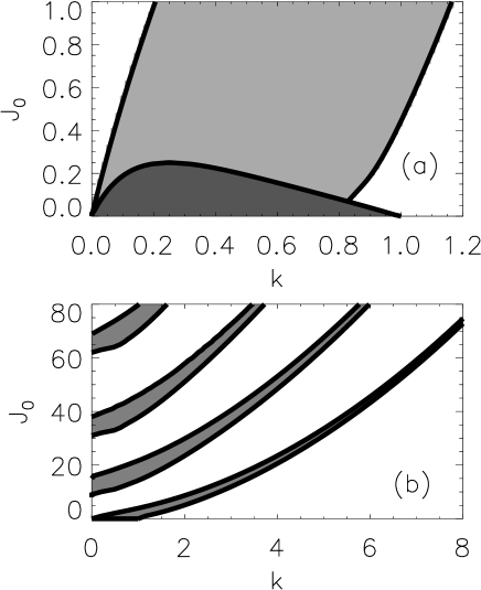
Figure 1: Stability diagram for the Hazel model for $R=3$. Panel (a) shows the Kelvin-Helmholtz unstable regions with dark gray, and Holmboe unstable regions with light gray. Panel (b) shows the same instability diagram for larger values of $J_{0}$.

A typical example used in many studies assumes a velocity profile given by $U(y)=\tanh(y)$ and the squared Brünt-Vaisala frequency being given by $J=J_{0}\cosh(Ry)^{-2}$. Where $J_{0}$ is the global Richardson number usually defined as $J_{0}\equiv\mathrm{Ri}(0)$. The case of $R=1$ was examined by Miles Miles (1963) analytically and numerically by Hazel Hazel (1972). It exhibits only Kelvin-Helmholtz instability for the wavenumbers that satisfy $k(1-k)>J_{0}$. Hazel Hazel (1972) also examined numerically the case $R=5$ where it was shown that along with the Kelvin-Helmholtz unstable region there is also a stripe (in a $J_{0}-k$ diagram) of unstable Holmboe modes. As an example the instability region for $R=3$ is shown in figure 1. Hazel observed that if $R>2$ there is always a height at which the local Richardson number is smaller than 1/4. Based on this observation Hazel conjectured that $R=2$ is the critical value of $R$ above which the Holmboe instability appears. Later careful numerical examination by Smyth Smyth & Peltier (1989) found unstable Holmboe modes to appears only for values of $R$ larger than $R>2.4$. More recently Alexakis Alexakis (2005) showed that the instability can be found for smaller values of $R$ up to $R=2.2$ making the conjecture by Hazel still plausible. More specifically Alexakis Alexakis (2005) showed (numerically) for the examined shear and density profiles that the left instability boundary of the Holmboe instability region (see figure 1a) is composed of marginally unstable modes with phase velocity equal to the maximum or the minimum of the shear velocity. Such a condition has been known to hold for smooth velocity and discontinuous density profiles Alexakis, Young & Rosner (2002, 2004); Churilov (2005). Finding these marginally unstable modes corresponds to solving a Schröndiger problem for a particle in a potential well:

$$\frac{d^{2}\phi}{dy^{2}}-\left[k^{2}+V_{c}(y)\right]\phi=0,$$ (3)

where

$$V_{c}(y)=\frac{U^{\prime\prime}}{U-c}-\frac{J(y)}{(U-c)^{2}}$$ (4)

and $c$ is taken to be $c=U_{\max/\min}$ the maximum or minimum velocity of the shear layer. The right boundary of the Holmboe unstable region on the other hand (see figure 1a) is composed of singular modes with phase velocity within the range of the shear velocity. These modes can be determined by imposing the condition that the solution close to the critical height can be expanded in terms of only one of the two corresponding Frobenius solutions. Furthermore it was shown that for sufficiently large $J_{0}$ more than one instability stripe exists. These new instability stripes are related with the higher internal gravity modes of the unforced system. Figure 1b shows the instability region for $R=3$ and $J_{0}$ up to $80$. We note that different unstable Holmboe modes have been found experimentally in Caulfield (1995) that were then interpreted in terms of the multi-layer model of Caulfield (1994).

The understanding however of the linear part of Holmboe instability for smooth shear and density profiles still remains conjectural and most of the results are based on numerical calculations and do not therefore constitute proofs. We try to address some of these issues in the present work. In the next section we prove for a general class of velocity profiles that the modes that have phase velocity equal to the maximum/minimum velocity of the shear are marginally unstable. In section III we examine the case for which the parameter $R$ is slightly larger than it’s critical value, and the dispersion relation inside the instability region is derived based on an asymptotic expansion. In section IV we test these results for specific shear and density profiles. A summary of the results and final conclusions are in the last section. To help the reader, a table 1 with the definitions of all the basic symbols used in this paper has been added.

Symbol	Definition
$c$	Complex phase velocity
$\zeta$	$=k{\mathrm{Im}}\{c\}$ the growth rate
$k$	Wavenumber
$\phi(y)$	Stream function
$k_{0}$	Wavenumber for which $c(k_{0})=U_{\infty}$
$\phi_{0}$	Stream function for the $c(k_{0})=U_{\infty}$ mode
$y_{c}$	Location of the critical layer $U(y_{c})=c$
$J_{0}$	Global Richardson Number
$U_{\infty},U_{*},\alpha$	Coefficients that appear in the large $y$
	behavior of $U(y)\simeq U_{\infty}-U^{*}e^{-\alpha y}$
$\beta,J_{*}$	Coefficients that appear in the large $y$
	behavior of $J(y)\simeq J^{*}e^{-\beta y}$
$\varphi_{\infty}$, $\lambda$	Coefficients that appear in the large $y$
	behavior of $\phi_{0}(y)\simeq\varphi_{\infty}e^{-\lambda y}$
$J_{\infty}$, $\sigma$, $R$, $q$	$J^{*}/(U^{*}\alpha)^{2}$, $\,\,U^{*}/U_{\infty}$, $\,\,\alpha/\beta$, $\,\,k/\alpha$
$\delta$	$=R-2$
$\tilde{J}$	=$J_{\infty}(\epsilon c_{1}/\sigma)^{\delta}$
	local Richardson number at $y=y_{c}$
$\mu$	$=1/2-\sqrt{1/4-\tilde{J}}$
$\lambda$	$=\sqrt{q^{2}+1-\tilde{J}}$
$F(a,b,d,s)$	Hypergeometric Function

Table 1: Table of used symbols

II Marginal wavenumber

In this section we examine modes with phase velocity equal to the maximum/minimum velocity of the flow, and show under what conditions these modes constitute a stability boundary. We start by considering an infinite shear layer specified by the monotonic velocity profile $U(y)$ that has the asymptotic values $U(\pm\infty)=U_{\pm\infty}$. Since the system is Galilean invariant with no loss of generality we can set $U_{+\infty}=-U_{-\infty}=U_{\infty}$. More precisely we will assume that the asymptotic behavior of $U(y)$ for $y\to+\infty$ is going to be given by

$$U(y)\simeq U_{\infty}-U_{*}e^{-\alpha y}.$$

We further assume that the layer is stably stratified with $J(y)>0$ having asymptotic behavior $J(y)\simeq J_{*}e^{-\beta y}$ for $y\to+\infty$. In what follows we are going to concentrate only on the modes with phase velocity close to $c=U_{\infty}$; the results can easily be reproduced for the $c=U_{-\infty}$ modes by following the same arguments. To simplify the problem we will non-dimentionalize the equations using the maximum velocity $U_{\infty}$ and the length-scale $\alpha^{-1}$ (essentially setting $U_{\infty}=1$ and $\alpha=1$). The resulting non-dimensional control parameters for our system are the asymptotic Richardson number:$J_{\infty}\equiv J_{*}/(U_{*}\alpha)^{2}$, the ratio of the two velocities:$\sigma\equiv U_{*}/U_{\infty}$, and the ratio of the two length scales: $R\equiv\beta/\alpha$. The wavenumber becomes $q=k/\alpha$ and $c$ is measured in units of $U_{\infty}$.

Finally we assume that a solution $\phi_{0}(y)$ of the Schröndiger problem described in equation 3 for the wavenumber $q_{0}=k_{0}/\alpha$ exists. Clearly if $R>2$ and $c=1$ the asymptotic behavior of $V_{c}$ for large $y$ is $V_{c}(y)\simeq 1$ and $\phi_{0}(y)$ behaves as $\phi\sim\varphi_{\infty}e^{-\lambda y}$ with $\lambda=\sqrt{q^{2}+1}$. If however we have $R=2$ then $V_{c}(y)\simeq 1-J_{\infty}$ for $y\to\infty$ and $\lambda=\sqrt{q^{2}+1-J_{\infty}}$. For abbreviation we will denote for both cases

$$\lambda=\sqrt{q^{2}+1-\tilde{J}}$$

where $\tilde{J}$ (that will be defined precisely later on) takes the values $\tilde{J}\simeq 0$ when $R>2$ and $\tilde{J}=J_{\infty}$ when $R=2$. As discussed in Alexakis (2005), no solution exists that satisfies the boundary conditions for the Schröndiger problem described in equation 3 if $R<2$ since it corresponds in finding bounded eigenstates in an unbounded potential well.

Our aim in this section is to find how $c$ changes from the value 1 as we increase $q$ from the value $q_{0}=k_{0}/\alpha$. We proceed by carrying out a regular asymptotic expansion by letting $q=q_{0}+\epsilon q_{1}$ and $c=1-\epsilon c_{1}+\dots$ with $\epsilon\ll 1$ and $c_{1}$ in general complex. However as we deviate from the $c=1$ solution the behavior of the potential $V_{c}(y)$ drastically changes ($\mathcal{O}(1)$ change) in the large $y$ region and only slightly (linearly with respect to the change in $c$) for $y\simeq{\mathcal{O}}(1)$. Figure 2 illustrates this change.

Figure 2: The potential $V_{c}$ for the Hazel model with $R=3$ and $J_{0}=1$ for three values of $c$, $c=1$ (solid line), $c=1+\epsilon$ (dashed line), $c=1-\epsilon$ (dotted line), where $0<\epsilon\ll 1$. For $c=1$ $V_{c}$ asymptotes to the value $V_{c}\simeq\alpha^{2}$. This behavior drastically changes when $c\neq 1$.

This implies that two different expansions are needed, one for $y$ being of ${\mathcal{O}}(1)$ and one for large $y$.

II.1 Local solution: $y={\mathcal{O}}(1)$

We begin with the local solution and expand $\phi$ as $\phi=\phi_{0}+\epsilon\phi_{1}+\dots\,$ . For $y={\mathcal{O}}(1)$ at first order we obtain:

$$\frac{d^{2}\phi_{1}}{dy^{2}}-\left[q_{0}^{2}+V_{0}(y)\right]\phi_{1}=\left[2q_{1}q_{0}-c_{1}V_{1}(y)\right]\phi_{0}$$ (5)

where $V_{0}=V_{c}$ is given in equation 4 for $c=1$ and

$$V_{1}(y)=\frac{\partial}{\partial c}\left[\frac{U^{\prime\prime}}{U-c}-\frac{J(y)}{(U-c)^{2}}\right]\Big{|}_{c=1}$$

$$=\frac{U^{\prime\prime}}{(U-1)^{2}}-\frac{2J(y)}{(U-1)^{3}}.$$

The solution of this inhomogeneous equation can be found using the Wronskian to obtain:

$$\phi_{1}=\phi_{0}(y)\int_{0}^{y}\frac{\int_{-\infty}^{y^{\prime}}[2q_{1}q_{0}-c_{1}V_{1}(y^{\prime\prime})]\phi^{2}_{0}(y^{\prime\prime})dy^{\prime\prime}}{\phi^{2}_{0}(y^{\prime})}dy^{\prime}$$ (6)

Where we have used as normalization condition $\phi(0)=\phi_{0}(0)$. Clearly this solution satisfies the boundary condition for $y\to-\infty$. For $y\to+\infty$, by performing the integrations we obtain:

$$\phi_{1}\simeq\frac{2q_{1}q_{0}I_{1}-c_{1}I_{2}}{\varphi_{\infty}}e^{\lambda y}+{\mathcal{O}}(e^{-\lambda y})$$ (7)

where $I_{1}=\int_{-\infty}^{+\infty}\phi^{2}_{0}dy>0$ and $I_{2}=\int_{-\infty}^{+\infty}V_{1}\phi^{2}_{0}dy.$ So the large $y$ behavior of $\phi$ based on the local solution is given by:

$$\phi\simeq\varphi_{\infty}e^{-\lambda y}+\epsilon\frac{2q_{1}q_{0}I_{1}-c_{1}I_{2}}{\varphi_{\infty}}e^{\lambda y}+\dots\,\,\,.$$ (8)

II.2 Far away solution: $y={\mathcal{O}}(\ln[1/\epsilon])$

To capture the large $y$ behavior we need to make the change of variables $\tilde{y}=y-y_{c}$ where $y_{c}=-\ln(\epsilon c_{1}/\sigma)$ is the location of the singularity determined by $U(y_{c})=c$. (Note that for $c_{1}$ complex $\tilde{y}$ does not coincide with the real $y$ axis.) The Taylor-Goldstein equation 1 then reads:

$$\frac{d^{2}\phi}{d\tilde{y}^{2}}-\left[q^{2}-\frac{1}{e^{\tilde{y}}-1}-\frac{J_{\infty}\cdot\left(\frac{\epsilon c_{1}}{\sigma}\right)^{\delta}\cdot\big{(}e^{-\tilde{y}}\big{)}^{\delta}}{(e^{\tilde{y}}-1)^{2}}\right]\phi=0$$ (9)

where $\delta=R-2$ and only the leading terms have been kept. Introducing the variable $s=e^{-\tilde{y}}$ we obtain:

$$s^{2}\frac{d^{2}}{ds^{2}}\phi+s\frac{d}{ds}\phi-\left[q^{2}-\frac{s}{1-s}-\frac{\tilde{J}s^{2}\,\,s^{\delta}}{(1-s)^{2}}\right]\phi=0,$$ (10)

where $\tilde{J}=J_{\infty}\cdot\left({\epsilon c_{1}}/{\sigma}\right)^{\delta}$ gives the Richardson number at the critical height. Note that if $R=2$ ($i.e.$ $\delta=0$) then $\tilde{J}=J_{\infty}={\mathcal{O}}(1)$. If however $R>2$ then $\tilde{J}\ll 1$ and the term in the brackets proportional to $\tilde{J}$ is small and can be neglected everywhere except close to the singularity $s=1$. To deal with this small singular term we can write for $s$ close to 1: $s^{\delta}\simeq 1-\delta(1-s)+\dots$ and keep the leading term. That way the principal term inside the brackets is always kept for all values of $s$ and our solution will be correct to first order for all values of $R\geq 2$ by solving:

$$s^{2}\frac{d^{2}}{ds^{2}}\phi+s\frac{d}{ds}\phi-\left[q^{2}-\frac{s}{1-s}-\frac{\tilde{J}s^{2}}{(1-s)^{2}}\right]\phi=0.$$ (11)

To deal with the singularities at $s=0$ and $s=1$ we make the substitution $\phi=s^{q}(1-s)^{\mu}h(s)$ with $\mu=1/2-\sqrt{1/4-\tilde{J}}$. We then obtain:

$$s(1-s)\frac{d^{2}}{ds^{2}}h+[(2q+1)-(2\mu+2q+1)s]\frac{d}{ds}h+$$

$$[1-\mu-(q+1)]h=0,$$ (12)

the solution of which is the Hypergeometric function $h(s)=F(a,b,d;s)$ with:

$${a}=(\mu+q)+\sqrt{q^{2}+1-\tilde{J}},$$

$${b}=(\mu+q)-\sqrt{q^{2}+1-\tilde{J}},$$

and

$${d}=(2q+1).$$

Note that $q+\mu-a=-\lambda$ and $q+\mu-b=+\lambda$. Some basic properties of the Hypergeometric function are given in appendix A, here we give just some of the resulting asymptotic behavior of $\phi$:

$$\lim_{s\to 0}\phi \simeq s^{q}=e^{-qy}$$ (13)

$$\lim_{s\to+\infty}\phi \simeq \frac{\Gamma(d)\Gamma(b-a)}{\Gamma(b)\Gamma(d-a)}s^{q}(-s)^{\mu-a}$$ (14)

$$+ \frac{\Gamma(d)\Gamma(a-b)}{\Gamma(a)\Gamma(d-b)}s^{q}(-s)^{\mu-b}.$$

Returning to the $y$ variable and up to a normalization factor $A$ we have for $y\ll y_{c}$ that

$$\phi\simeq A\left[e^{-\lambda y}+(-\epsilon c_{1})^{2\lambda}\frac{\Gamma(a)\Gamma(d-b)\Gamma(-2\lambda)}{\Gamma(b)\Gamma(d-a)\Gamma(2\lambda)}e^{\lambda y}\right].$$ (15)

II.3 Matching

Matching the exponentially decreasing terms of the local and the far-away solution we obtain: $A=\varphi_{\infty}$, and from the exponentially increasing terms we have:

$$\epsilon\frac{2q_{1}q_{0}I_{1}-c_{1}I_{2}}{\varphi_{\infty}}=\varphi_{\infty}(-\epsilon c_{1})^{2\lambda}\frac{\Gamma(a)\Gamma(d-b)\Gamma(-2\lambda)}{\Gamma(b)\Gamma(d-a)\Gamma(2\lambda)}.$$ (16)

We can solve the equation above iteratively by letting $\epsilon c_{1}=\epsilon c^{\prime}_{1}+\epsilon^{2\lambda}c^{\prime}_{2}+\dots\,\,\,$. To first order we obtain:

$$c^{\prime}_{1}=\frac{2q_{1}q_{0}I_{1}}{I_{2}},$$ (17)

which gives the first correction to the phase speed and determines if the real part of phase speed is increasing or decreasing with the wavenumber. If for example $I_{2}>0$ (which will be the case in the examples that follow) then $c$ is decreasing with $q$ and the correction $c_{1}^{\prime}$ is positive for positive $q_{1}$ and negative for negative $q_{1}$. The opposite holds if $I_{2}<0$. From now on we will assume that $I_{2}>0$ which is the physically relevant case (Re$\{c(k)\}$ being a decreasing function of $k$) if however there is a velocity and density profile such that $I_{2}<0$ the same results will hold but for the opposite direction in $q$ ($i.e.$ wavenumbers smaller than $q_{0}$ will be unstable and wavenumbers larger than $q_{0}$ will be stable). The $c_{1}^{\prime}$ correction however is real, and contains no information about the growth rate. At the next order we have

$$-c^{\prime}_{2}I_{2}/\varphi_{{}_{\infty}}=\varphi_{\infty}(-c^{\prime}_{1})^{2\lambda}\frac{\Gamma(a)\Gamma(d-b)\Gamma(-2\lambda)}{\Gamma(b)\Gamma(d-a)\Gamma(2\lambda)}.$$ (18)

This correction is much smaller but contains the first order correction of the imaginary part of $c$. The dispersion relation of $c$ for $q$ close to $q_{0}$ can then be written in terms of $q$ as:

$$c=1-\frac{2q_{0}I_{1}}{I_{2}}(q-q_{0})+\qquad$$

$$\frac{{\varphi_{{}_{\infty}}}^{2}}{I_{2}}\left(\frac{-2k_{0}I_{1}}{I_{2}}(q-q_{0})\right)^{2\lambda}\frac{\Gamma(a)\Gamma(d-b)\Gamma(-2\lambda)}{\Gamma(b)\Gamma(d-a)\Gamma(2\lambda)}$$ (19)

Special care is needed to interpret the term $(-c_{1}^{\prime})^{2\lambda}$ for $c_{1}^{\prime}$ is given by equation 17. When $q_{1}<0$, $c_{1}^{\prime}$ is negative and the term $(-c_{1}^{\prime})^{2\lambda}$ is real, this corresponds to the case that $c$ becomes larger than the shear velocity and no critical layer is formed. The Howard semi-circle theorem then guaranties stability. This proves that wavenumbers slightly smaller than $q_{0}$ are stable. When $q_{1}>0$, $c_{1}^{\prime}$ is positive and $(-c_{1}^{\prime})^{2\lambda}$ becomes a complex number that can take different values depending on whether the minus sign is interpreted as $e^{i\pi}$ or $e^{-i\pi}$. The choice depends on the location of the singularity on the complex plane when we integrate the Taylor Goldstein equation 1. If Im$\{c_{1}\}>0$ then $(-c_{1})^{2\lambda}$ should be interpreted as $|c_{1}|^{2\lambda}\,\,e^{-i2\lambda\pi}$ because the integration is going over the singularity. If Im$\{c_{1}\}<0$ then $(-c_{1})^{2\lambda}$ should be interpreted as $|c_{1}|^{2\lambda}\,\,e^{+i2\lambda\pi}$ because the integration is going under the singularity. Here we arrive at an important point in our derivation: the sign of the imaginary part of $c$ based on equation 19 depends on the original assumption about the sign of Im$\{c\}$ when we integrate across the singularity. Thus, in order for the matching to be successful we need to verify that the original assumption about the sign of Im$\{c_{1}\}$ is consistent with the final result. If we assume that Im$\{c_{1}\}>0$ then from 18 we have that

$$0<{\mathrm{Im}}\{c_{1}\}=\sin(2\lambda\pi)|c_{1}|^{2\lambda}\frac{\varphi_{\infty}^{2}}{I_{2}}\frac{\Gamma(a)\Gamma(d-b)\Gamma(-2\lambda)}{\Gamma(b)\Gamma(d-a)\Gamma(2\lambda)}$$ (20)

where Im$\{(c_{1}^{\prime})^{2\lambda}\}$ is written as $-\sin(2\lambda\pi)|c_{1}|^{2\lambda}$ as previously discussed. The matching is successful only if the sign of the right hand side ($r.h.s.$) of equation 20 is positive as originally assumed and only then is the dispersion relation 19 valid. (We arrive at the same condition if we initially assume that Im$\{c\}<0$). It is shown in appendix B that for $R>2$ (i.e. $\tilde{J}\simeq 0$) the $r.h.s.$ of 20 is always positive and the matching is successful. For the special case however that $R=2$ (i.e. $\tilde{J}=J_{\infty}$) the matching is not always successful because the product $\Gamma(b)\Gamma(d-a)$ that appears in equation 20 can change sign depending on the value of $\tilde{J}$. In particular it is shown in the appendix that if $\tilde{J}>2q/(2q+1)^{2}$ the $r.h.s.$ of equation 20 is negative and thus we end up with a contradiction. Therefore in the $R=2$ case we have shown instability only if

$$\tilde{J}<2q/(2q+1)^{2}.$$ (21)

The unsuccessful matching when the condition 21 is not satisfied suggests that the modes with $q>q_{0}$ are part of the continuous spectrum of the Taylor Goldstein equation. This kind of modes have a discontinuity of the first derivative of $\phi$ at the critical layer and have been studied before in the literature Banks, Drazin & Zaturska (1976); Balmforth (1995). We need to emphasize here that the lack of instability at this order does not imply stability. Non-zero growth rate of smaller order can still exist and therefore the above result should be interpreted only as a sufficient condition for instability.

To summarize we have shown that if $R>2$ the modes with phase velocity equal to the maximum phase velocity of the shear (when they exist, and for density and velocity profiles that satisfy the conditions stated at the beginning of this section) are marginally unstable: wavenumbers with $q<q_{0}$ are stable and wavenumbers with $q>q_{0}$ are unstable. If $R=2$ these modes are marginally unstable only if the condition 21 is further satisfied and stable (to the examined order) otherwise.

III Marginal R

In the last sectioned we showed marginal instability when the wavenumber $q$ is varied from the critical value $q_{0}$. However the wavenumber is not a control parameter in a system. We would like therefore to examine a system for which one of the control parameters ($J_{0}$ or $R$) is close to the critical value for which the instability begins. Since Holmboe instability is present for arbitrary large values of $J_{0}$ the only other control parameter left is $R$. We consider therefore a case for which $R=2+\delta$ with $0<\delta\ll 1$ and the $c=1$ solution ($\phi_{0},q_{0})$ is known with $q_{0}$ such that $J_{\infty}>2q_{0}/(2q_{0}+1)^{2}$ so that the $R=2$ case gives no instability at the examined order. We make a small variation in $q=q_{0}+\epsilon q_{1}$ and $c=1-\epsilon c_{1}$ with the exact relation between $\delta$ and $\epsilon$ still undetermined. At this stage we assume that $\epsilon$ is sufficiently smaller than $\delta$ so that the procedure in the previous section is still valid and then gradually increase its value until the approximations in the previous section start to fail. As we increase the value of $\epsilon$ the most sensitive term (in $\epsilon$) that will be affected first, is the term proportional to $\tilde{J}=J_{\infty}\cdot\left({\epsilon c_{1}}/\sigma\right)^{\delta}$ in the equation 11 for which $\epsilon$ is raised to the smallest appearing power. Note that if $\epsilon\ll\exp[-1/\delta]$ then $\tilde{J}\ll 1$ and the results of the previous section are still valid. If however $\epsilon\sim{\mathcal{O}}(\exp[-1/\delta])$ then $\tilde{J}\sim{\mathcal{O}}(1)$. Following the same steps as in the previous section we end up in the dispersion relation given by equation 19 but like in the $R=2$ case $\tilde{J}$ cannot be treated as a small parameter.

The difference from the $\delta={\mathcal{O}}(1)$ case will therefore appear when we try to determine the sign of the $r.h.s.$ of equation 20. To have successful matching we need to satisfy the condition 21. Since $\tilde{J}$ is finite the condition $\tilde{J}<2q/(2q+1)^{2}$ that also appears in the $R=2$ case could be violated. To capture the whole unstable region we define $\epsilon$ such that $J_{\infty}\epsilon^{\delta}=2q_{0}/(1+2q_{0})^{2}$ or

$$\epsilon=\left[\frac{2q_{0}/J_{\infty}}{(1+2q_{0})^{2}}\right]^{1/\delta}\ll 1.$$ (22)

Note that the term inside the brackets is always smaller than one. For such a choice the condition 21 for instability reads

$$\tilde{J}=J_{\infty}\cdot\left(\frac{\epsilon c_{1}}{\sigma}\right)^{\delta}=$$

$$\left[\frac{2q_{0}}{(1+2q_{0})^{2}}\right][1+\delta\ln(c_{1}/\sigma)+\mathcal{O}(\delta^{2})]$$

$$<\left[\frac{2q_{0}}{(1+2q_{0})^{2}}\right]+\mathcal{O}(\epsilon)$$ (23)

or $c_{1}/\sigma<1$. Already at this stage it can be seen that we have instability only if $c_{1}=2q_{1}q_{0}I_{1}/I_{2}<\sigma$ and therefore the instability is confined in the region of wave numbers

$$q_{0}<q<q_{0}+\Delta q$$ (24)

where $\Delta q=\epsilon\sigma I_{2}/2q_{0}I_{1}$. Therefore, the second instability boundary for the Holmboe instability is given by $q+\Delta q$. To get the full dispersion relation in this asymptotic limit we need to expand in terms of $\delta$ the product $\Gamma(d-a)\Gamma(b)$ that appears in equation 19 since this is the term that can change sign depending on the value of $\tilde{J}$. This is done in Appendix B and the resulting growth rate inside the instability region to the first non-zero order becomes:

$$\zeta=q_{0}{\mathrm{Im}}\{c\}=-{\delta C_{1}q_{0}}|q_{0}-q|^{2\lambda}\ln\left(\frac{2(q-q_{0})q_{0}I_{1}}{\epsilon I_{2}\sigma}\right)$$ (25)

where $C_{1}>0$ is an ${\mathcal{O}}(1)$ quantity and is given in equation 28. The maximum of the growth rate is obtained for $q-q_{0}=\epsilon e^{-1/2\lambda}I_{2}\sigma/(2q_{0}I1)$ with the growth rate being given by:

$$\max{[\zeta]}=\delta\epsilon^{2\lambda}\frac{C_{1}q_{0}\lambda}{2\lambda e}\left[\frac{I_{2}\sigma}{q_{0}I_{1}}\right]^{2\lambda}$$ (26)

Therefore the growth rate scales like $\epsilon^{2\lambda}$ and the width of the instability region scales like $\Delta q\sim\epsilon$. In terms of $\delta$ these relations are given by $\zeta\sim\delta e^{-2\lambda\gamma/\delta}$ and $\Delta q\sim e^{-\gamma/\delta}$ where $\gamma$ is a positive constant. This very strong dependence with $\delta$ suggests that both $\zeta$ and $\Delta q$ decrease very rapidly as $\delta$ becomes smaller. This can explain the difficulty numerical codes have, when attempting to calculate growth rate for values of $R$ very close to $R=2$.

IV Examples

In the previous sections we showed some general results for the Holmboe unstable modes. In this section we examine some specific examples often used in the literature to model Holmboe’s instability. We begin with the model introduced by Hazel that we briefly mentioned in the introduction. The model assumes a velocity profile given by $U(y)=\tanh(y)$ and a density stratification determined by $-g\rho^{\prime}/\rho=J_{0}\cosh^{-2}(Ry)$. Based on the definitions given in section II we have that $\alpha=2$, $\beta=2R$, $U_{*}=2$ and $J_{*}=4J_{0}$. The resulting non-dimensional quantities are $J_{\infty}=J_{0}/4$, $\sigma=2$, $q=k/2$ and $R$ has the same meaning. This model satisfies all the conditions that are stated in section II therefore for $R>2$ the modes with $c(k)=\pm 1$ are marginally unstable. Furthermore for the case $R=2$ we will have instability only if the condition 21 is satisfied, or in the units of this example if $J_{0}/4<k/(k+1)^{2}$. A simple numerical integration shows that this is not the case for this profile (see figure 3).

Figure 3: The $c=1$ solutions for the Hazel model $J_{0}(k)$ for $R=2$ (solid line), the condition from equation 21 $J_{0}<4k/(k+1)^{2}$ (dashed line).

Therefore, the $R=2$ is stable (to the examined order) and is the critical value beyond which the Holmboe instability begins. The imaginary part of $c(k)$ for this profile for the case that $R=2.1$ and $J_{0}=1.2$ is shown if figure 4 where the numerical result is compared with the asymptotic expansion of equation 25. Although $\delta=0.1$ is not very small there is satisfactory agreement (a 20% difference) between the asymptotic and the numerical result. It is worth mentioning that it is very hard to find a range of values of $\delta$ that both the asymptotic result is valid and Im$\{c\}$ is large enough to be captured by a numerical code. Note that by decreasing the value of $\delta$ from $0.1$ to $0.05$ has resulted in a drop of Im$\{c\}$ by three orders of magnitude.

Figure 4: The Im$\{c\}$ for the Hazel model for $R=2+\delta$ with $\delta=0.1,\,0.75,\,0.05$ and $J_{0}=1.2$. The diamonds indicate the results from numerical integration for the $\delta=0.1$ case.

A second family of flows we will examine assumes a velocity profile given by $U(y)=\tanh(y)$ as in the Hazel model and the density stratification being determined by:

$$-g\rho^{\prime}/\rho=\frac{J_{0}}{\cosh^{2R}(y)}.$$

The advantage of this profile is that there are analytic solutions for the Kelvin-Helmholtz stability boundaries $J_{0}(k)$ for the cases that $R=0,1$ and $2$. In addition there is an analytic solution $J_{0}(k)$ for the modes $k$ for which $c(k)=1$ for the $R=2$ case. The $R=0$ case was examined by Drazin (1958) where it was shown that the Kelvin Helmholtz unstable modes satisfy $J_{0}<k^{2}(1-k^{2})$. The $R=1$ case (that reduces to the $R=1$ case of the Hazel model) was investigated by Miles (1963) where it was shown that the Kelvin Helmholtz unstable modes satisfy $J_{0}<k(1-k)$. The $R=2$ case has not been investigated before (to the author’s knowledge). One can show following the same methods used for the $R=0,1$ cases Drazin (1958); Miles (1963); Howard (1963) that the $c(k)=0$ modes satisfy:

$$J_{0}=\frac{k(1-k)(2+k)(3+k)}{4(k+1)^{2}}$$

with $\phi(y)=[1-\tanh(y)^{2}]^{k/2}\cdot[\tanh(y)]^{1/4-\sqrt{1/4-J_{0}}}$ and provide the Kelvin-Helmholtz instability boundary. $c(k)=1$ modes on the other hand that are of interest for the Holmboe instability satisfy

$$J_{0}=\frac{k(3+2k)}{(k+1)^{2}}$$

for $k<1$. The stream-function $\phi$ for these modes is given by $\phi=[1+\tanh(y)]^{k/2}\cdot[1-\tanh(y)]^{\sqrt{k^{2}/4+1-J_{0}}}$. The Kelvin-Helmholtz stability boundaries for the three cases $R=0,1,2$ along with the $c=1$ solutions for the $R=2$ case are shown in figure 5.

Figure 5: The $c=1$,and $c=0$ solutions for the model with density stratification given by $J(y)=J_{0}\cosh^{-2R}(y)$ for $R=0$ (dotted line), $R=1$ (dotted line), $R=2$ (solid line).

For this example we also have that $\sigma=2$ and $q=k/2$ but $J_{\infty}=2^{2R-4}J_{0}$. The $J_{0}(k)$ relation for the $c=1$ solutions does not satisfy the criterion 21 that now reads $J_{0}<k/(k+1)^{2}$, thus the $R=2$ case is stable (to the examined order) and is the critical value above which the Holmboe instability begins. Because $J_{\infty}$ is four times bigger than in the Hazel model (for the same $J_{0}$) the resulting growth rate is smaller by a factor of $4^{-2\lambda/\delta}$ that is close to $10^{-14}$ for the $\delta=0.1$ case. Figure 6 shows the growth rate based on the asymptotic expansion 25. No numerical results could be obtained for this case for values of $\delta$ smaller than $\delta\leq 0.1$ that would justify a comparison with the asymptotic expansion.

Figure 6: The Im$\{c\}$ for the $J(y)=J_{0}\cosh^{-2R}(y)$ model for $J_{0}=1.2$ and $R=2+\delta$ with $\delta=0.1$ (solid line) and $\delta=0.075$ (dashed line).

This example, when compared with one of Hazel, clearly demonstrates the sensitivity of the resulting growth rate to the large $y$ asymptotic behavior of $J(y)$ and $U(y)$: a change by a factor of $4$ in $J_{\infty}$ resulted in 14 orders of magnitude difference in the growth rate.

V Conclusions

In this paper we have examined analytically Holmboe’s instability for smooth density and velocity profiles. We have shown for a large family of flows that the modes with phase velocity equal to the maximum or minimum of the unperturbed velocity profile when they exist and if the parameter $R$ is above the critical value ($R_{crit}=2$) they constitute a stability boundary. This result confirms the results obtained numerically in Alexakis (2005) where the fact that the $c=U_{\max/\min}$ modes are marginally unstable was only conjectured based on physical arguments. It is also the first time shown analytically that the value of $R=2$ for the Hazel model is the critical value $R_{crit}$ above which the Holmboe instability begins.

For the case that the parameter $R$ is only slightly larger than it’s critical value $R_{crit}=2$, the dispersion relation $c(k)$ was obtained based on an asymptotic expansion. For this marginally unstable flow the growth rate $\zeta$ as well as the width of the instability stripe $\Delta q$ have a very strong dependence on the deviation of $R$ from it’s critical value. In particular the growth rate $\zeta$ and the width of the instability $\Delta k=$ scale as $\exp[-2\lambda\gamma/(R-R_{crit})]$ and $\exp[-\gamma/(R-R_{crit})]$ respectively (for some positive constant $\gamma$). For this reason the numerical investigations performed in the past Smyth & Peltier (1989); Alexakis (2005) were not able to capture the instability for values of $R$ very close to $R_{crit}$.

We believe also that the present results go beyond the clarifying of a mathematical detail in the literature. They clearly demonstrate the nature of the Holmboe instability in a quantitative way. The critical layer for Holmboe unstable modes appears at large heights where the shear rate can overcome stratification and the behavior mode will strongly depend on the properties of the shear at this height. The critical layer is then coupled to the gravity wave modes that their properties are determined by $y={\mathcal{O}}(1)$ quantities and are fast enough to travel with the same velocity as the velocity at the critical layer height. It is this coupling that gives rise to the instability, and it is restricted only to the wave numbers that result in a phase speed that is smaller than the maximum velocity of the shear but big enough so that the critical layer is at a large enough height so that $Ri(y)<1/4$. Therefore in any experimental setup, precise measurements of the velocity and density stratification are needed in both large and small heights in order to make comparisons of the measured growth rate and the theoretical predictions.

Finally we believe that the results given in this paper can provide a basis for further numerical and analytical investigations such as an examination of the weakly non-linear theory where a small non-linearity is taken into account in order to examine the long time evolution of an unstable mode beyond the linear stage.

Appendix A The Hyper-geometric equation: Basic Properties

The Hypergeometric equation is:

$$z(1-z)\frac{d^{2}f}{dz^{2}}+[d-(a+b+1)z]\frac{df}{dz}-abf=0.$$ (27)

The solution that remains finite as $z\to 0$ is the Hypergeometric function: $f=F(a,b,c;z)$. For the normalization condition we are using we have the following limits:

$$\lim_{z\to 0}F(a,b,c;z) = 1/\Gamma(d)$$

$$\lim_{z\to 1}F(a,b,c;z) \simeq \frac{\Gamma(d)\Gamma(d-a-b)}{\Gamma(d-a)\Gamma(d-b)}$$

$$+ \frac{\Gamma(d)\Gamma(a+b-d)}{\Gamma(a)\Gamma(b)}(1-z)^{d-a-b}$$

$$\lim_{z\to+\infty}F(a,b,c;z) \simeq \frac{\Gamma(d)\Gamma(b-a)}{\Gamma(b)\Gamma(d-a)}(-z)^{-a}$$

$$- \frac{\Gamma(d)\Gamma(a-b)}{\Gamma(a)\Gamma(d-b)}(-z)^{-b}$$

provided that $d\neq 0,-1,-2,\dots$ and $a-b$ is not an integer.

Appendix B The sign of the instability term

To determine whether we have successful matching or not we need to find the sign of the imaginary part in the dispersion relation 19. We examine each term separately. Clearly $\Gamma(a)$, $\Gamma(2\lambda)$ and $\Gamma(d-b)$ are all positive factors since the argument of the $\Gamma$-function is positive. The factor $\Gamma(-2\lambda)$ is changing sign every time $2\lambda$ is an integer. However its product with $\sin(2\lambda\pi)$ is always remains negative. The factors $\Gamma(b)$ and $\Gamma(d-a)$ however can change sign depending on value of $\tilde{J}$. Using the expressions for $a,b,d$ one can show that $-1\leq b\leq 0$ if $\tilde{J}\leq(2q)/(2q+1)^{2}$ or if $2q\leq 1$, and positive otherwise. Similarly we have that $-1\leq d-a<0$ if $\tilde{J}>(2q)/(2q+1)^{2}$ and $2q<1$ and non-negative otherwise. Combining these two inequalities we can determine the sign of the product

$$\Gamma(b)\Gamma(d-a)\leq 0{\mathrm{\,if\,and\,only\,if\,}}\tilde{J}\leq(2q)/(2q+1)^{2}.$$

The result in 20 then follows.

To find the dispersion relation for the small $\delta$ and $\epsilon$ given by 22 we need to find an expression for the term $\Gamma(b)\Gamma(d-a)$. Substituting the choice of $\epsilon$ given by 22 in the expression for $b$ and $d-a$ and using $\tilde{J}=J_{\infty}(\epsilon c_{1}/\sigma)^{\delta}\simeq J_{\infty}(\epsilon)^{\delta}(1+\delta\ln(c_{1}/\sigma))$ we have that to first order in $\delta$ if $2q_{0}>1$:

$$b\simeq\frac{1}{2}\delta J_{\infty}\epsilon^{\delta}\ln(c_{1}/\sigma)\left[\frac{1}{\sqrt{1/4-J_{\infty}\epsilon^{\delta}}}+\frac{1}{\sqrt{1+q_{0}-J_{\infty}\epsilon^{\delta}}}\right]$$

and $b={\mathcal{O}}(1)$ if $2q_{0}<1$. Similarly,

$$d-a\simeq\frac{1}{2}\delta J_{\infty}\epsilon^{\delta}\ln(c_{1}/\sigma)\left[\frac{1}{\sqrt{1/4-J_{\infty}\epsilon^{\delta}}}+\frac{1}{\sqrt{1+q_{0}-J_{\infty}\epsilon^{\delta}}}\right]$$

if $2q<1$ and $d-a={\mathcal{O}}(1)$ if $2q>1$. Using the $\Gamma$-function property $\Gamma(\delta)=\Gamma(1+\delta)/\delta$ we can write the dispersion relation for $q_{0}<q<q_{0}+\epsilon\sigma I_{2}/k_{0}I_{1}$ as:

$$c=1-2(q-q_{0})q_{0}I_{1}/I_{2}+\delta C_{1}(q_{0}-q)^{2\lambda}\ln\left(\frac{2(q-q_{0})q_{0}I_{1}}{I_{2}\sigma}\right)$$

where

$$C_{1}=\frac{J_{\infty}\epsilon^{\delta}{\varphi_{{}_{\infty}}}^{2}}{2I_{2}}\left(\frac{2q_{0}I_{1}}{I_{2}}\right)^{2\lambda}\frac{\sin(2\lambda)\Gamma(a)\Gamma(d-b)\Gamma(-2\lambda)}{\Gamma(w)\Gamma(2\lambda)}\times$$

$$\left[\frac{1}{\sqrt{1/4-J_{\infty}\epsilon^{\delta}}}+\frac{1}{\sqrt{1+q_{0}-J_{\infty}\epsilon^{\delta}}}\right]$$ (28)

with $w=b$ if $2q_{0}<1$ and $w=d-a$ if $2q_{0}>1$.

References

- Rosner, Alexakis, Young, Truran & Hillebrand (2002) R. Rosner, A. Alexakis, Y. Young, J. Truran & W. Hillebrand, “On the C/O enrichment of novae ejecta”. Astrophys. J. 562, L177–L179 (2002).
- Alexakis (2004) A. Alexakis, A.C. Calder, A. Heger, E.F. Brown, L.J. Dursi, J.W. Truran, R. Rosner, D.Q. Lamb, F.X. Timmes, B. Fryxell, M. Zingale, P.M. Ricker, K. Olson, “On heavy element enrichment in classical novae” Astrophys. J. 603, 931–937 (2004).
- Farmer & Freeland (1983) D. M. Farmer & H. Freeland, “The physical oceanography of fjords,” Prog. Oceanogr. 12, 147 (1983).
- Pawlak & Armi (1997) G. Pawlak & L. Armi, “Hydraulics of two-layer arrested wedge flows,” J. Hydraul. Res. 35, 603 (1997).
- Armi & Farmer (1988) L. Armi & D.M. Farmer, “The flow of Mediterranean water through the Strait of Gibraltar”. Prog. Oceanogr. 21, 1–105 (1988).
- Oguz, Ozsoy, Latif, Sur, & Unluata (1990) T. Oguz, E. Ozsoy, M.A. Latif, H.I. Sur & U. Unluata, “Modeling of hydraulically controlled exchanged flow in the Bosphorous Strait”. J. Phys. Oceanogr. 20, 945–965 (1990).
- Sargent & Jirka (1987) F.E. Sargent & G.H. Jirka, “Experiments on saline wedge”. J. Hydraulic Eng. 113, 1307–1324 (1987).
- Yoshida, Ohtani, Nishida & Linden (1998) S. Yoshida, M. Ohtani, S. Nishida & P.F. Linden, “Mixing processes in a highly stratified river”. Physical Processes in Lakes and Oceans, edited by J. Imberger (American Geophysical Union, Washington DC, 1998)
- Pettre & Andre (1991) P. Pettre & J. C. Andre, “Surface-pressure change through Loewe’s phenomena and katabatic flow jumps. Study of two cases in Adelie Land Antartica,” J. Atmos. Sci. 48, 557–571 (1991).
- Holmboe (1962) J. Holmboe, “On the behavior of symmetric waves in stratified shear layers”. Geophys. Publ. 24, 67–113 (1962).
- Lawrence, Browand & Redecopp (1991) G.A. Lawrence, F.K. Browand & L.G. Redecopp, “The stability of a sheared density interface”. Phys. Fluids-A. 3, 2360–2370 (1991).
- Caulfield (1994) C.P. Caulfield, “Multiple linear instability of layered stratified shear flow”. J. Fluid Mech. 258, 255–285 (1994).
- Haigh & Lawrence (1999) S.P. Haigh & G.A. Lawrence, “Symmetric and non-symmetric Holmboe instabilities in an inviscid flow”. Phys. Fluids 11, 1459–1468 (1999).
- Ortiz, Chomaz& Loiseleux (2002) S. Ortiz, J.M. Chomaz & T. Loiseleux “Spatial Holmboe instability”. Phys. Fluids 14, 2585-2597 (2002).
- Hazel (1972) S.P. Hazel, “Numerical studies of the stability of inviscid shear flows”. J. Fluid Mech. 51, 3261–3280 (1972).
- Smyth & Peltier (1989) W.D. Smyth, & W.R. Peltier, “The transition between Kelvin-Helmholtz and Holmboe instability; An investigation of the over-reflection hypothesis”. J. Atmos. Sci. 46, 3698–3720 (1989).
- Alexakis (2005) A. Alexakis “On Holmboe’s instability for smooth shear and density profiles”. Phys. Fluids 17, 084103 (2005).
- Nishida & Yoshida (1987) S. Nishida & S. Yoshida, “Stability and eigenfunctions of disturbances in stratified two layer shear flow”. Proc. Third Intl. Symp. on Stratified Flows, Pasadena, California, 3-5 February 1987 pp.28–34
- Smyth, & Peltier (1990) W.D. Smyth & W.R. Peltier, “Three-dimensional primary instabilities of a stratified dissipative, parallel flow”. Geophys. Astrophys. Fluid Dyn. 52, 249–261 (1990).
- Smyth, Klaasen & Peltier (1988) W.D. Smyth, G.P. Klaasen & W.R. Peltier, “Finite amplitude Holmboe waves,”. Geophys. Astrophys. Fluid Dyn.. 43, 181–222 (1988).
- Smyth, & Peltier (1991) W.D. Smyth & W.R. Peltier, “Instability and transition in finite amplitude Kelvin-Helmholtz and Holmboe waves”. J. Fluid Mech. 228, 387–415 (1991).
- Sutherland, Caulfield & Peltier (1994) B.R. Sutherland, C.P. Caulfield & W.R. Peltier, “Internal gravity generation and hydrodynamic instability”. J. Atmos. Sci. 51, 3261–3280 (1994).
- Alexakis (2004) A. Alexakis, A.C. Calder, L.J. Dursi, R. Rosner, J.W. Truran, B. Fryxell, M. Zingale, F.X. Timmes, K. Olson, P. Ricker “On the nonlinear evolution of wind-driven gravity waves” Phys. Fluids 16, 3256–3268 (2004).
- Smyth, & Winters (2003) W.D. Smyth & K.B. Winters, “Turbulence and mixing in Holmboe waves”. J. Phys. Oceanogr.. 33, 694–711 (2003).
- Browand & Winant (1973) F.K. Browand & C.D. Winant “Laboratory observations of shear layer instability in a stratified fluid.” Boundary Layer Met. 5, 67–77 (1973).
- Koop (1976) C.G. Koop, “Instability and turbulence in a stratified shear layer”. Tech. Rep. USCAE 134 Department of Aerospace Engineering University of South California. (1976)
- Pawlak (1999) G. Pawlak & L. Armi, “Vortex dynamics in a spatially accelerating shear layer,” J. Fluid Mech. 376, 1– (1999).
- Pouliquen, Chomaz & Huerre (1994) O. Pouliquen, J.M. Chomaz & P. Huerre, “Propagating Holmboe waves at the interface between two immiscible fluids”. J. Fluid Mech. 266, 277–409 (1994).
- Zhu & Lawrence (2001) D.Z. Zhu & G.A. Lawrence, “Holmboe’s instability in exchange flows”. J. Fluid Mech. 429, 391–409 (2001).
- Hogg & Ivey (2003) A.M. Hogg & G.N. Ivey, “The Kelvin-Helmholtz to Holmboe instability transition in stratified exchange flows”. J. Fluid Mech. 477, 339–362 (2003).
- Yonemitsu, Swaters, Rajaratnam & Lawrence (1996) N. Yonemitsu, G.E. Swaters,N. Rajaratnam & G. A. Lawrence “Shear instabilities in arrested salt wedge flows”. Dyn. Atm. Oceans 24, 173–182 (1996).
- Caulfield (1995) C.P. Caulfield, W.R. Peltier, S. Yoshida & M. Ohtani “An experimental investigation of the instability of a shear flow with multilayered dencity stratification”. Phys. Fluids7,3028–3041 (1995).
- Drazin & Reid (1981) P.G. Drazin & W.H. Reid “Hydrodynamic Stability” Cambridge University Press (1981)
- Howard (1961) L.N. Howard, “A note on a paper of John Miles”. J. Fluid Mech. 10, 509–512 (1961).
- Miles (1963) J. Miles “On the stability of heterogeneous shear flow Part 2”. J. Fluid Mech. 16, 209–227 (1963).
- Alexakis, Young & Rosner (2002) A. Alexakis, Y. Young & R. Rosner “Shear instability of fluid interfaces: a linear analysis”. Phys. Rev. E. 65, 26313 (2002).
- Alexakis, Young & Rosner (2004) A. Alexakis, Y. Young & R. Rosner, “Weakly non-linear analysis of wind driven gravity waves”. J. Fluid Mech. 503, 171–200 (2004).
- Churilov (2005) S.M. Churilov “Stability analysis of stratified shear flows with a monotonic velocity profile without inflection points” J. Fluid Mech. 539, 25–55 (2005).
- Banks, Drazin & Zaturska (1976) W.H.H. Banks, P.G. Drazin & M.B. Zaturska “On the normal modes of parallel flow of inviscid stratified fluid”. J. Fluid Mech. 75, 149–171 (1976).
- Balmforth (1995) N.J. Balmforth & P.J. Morrison “Normal modes and continuous spectra” Annals of the New York Academy of Science 773 80–94 (1995)
- Drazin (1958) P.G. Drazin “The stability of a shear layer in an unbounded heterogeneous inviscid fluid”. J. Fluid Mech.4,214–224 (1958).
- Howard (1963) L.N. Howard, “Neutral curves and stability boundaries in stratified shear flow”. J. Fluid Mech. 16, 333–342 (1963).