How to Derive the Schrödinger Equation

Abstract

We illustrate a simple derivation of the Schrödinger equation, which requires only knowledge of the electromagnetic wave equation and the basics of Einstein’s special theory of relativity. We do this by extending the wave equation for classical fields to photons, generalize to non-zero rest mass particles, and simplify using approximations consistent with non-relativistic particles.

I Introduction

One of the most unsatisfying aspects of any undergraduate quantum mechanics course is perhaps the introduction of the Schrödinger equation. After several lectures motivating the need for quantum mechanics by illustrating the new observations at the turn of the twentieth century, usually the lecture begins with: “Here is the Schrödinger equation.” Sometimes, similarities to the classical Hamiltonian are pointed out, but no effort is made to derive the Schrödinger equation in a physically meaningful way. This shortcoming is not remedied in the standard quantum mechanics textbooks either griffiths ; merzbacher ; sakurai . Most students and professors will tell you that the Schrödinger equation cannot be derived. Beyond the standard approaches in modern textbooks there have been several noteworthy attempts to derive the Schrödinger equation from different principles hall ; peice ; field ; ogborn , including a very compelling stochastic method nelson , as well as useful historical expositions bernstein .

In this paper, we illustrate a simple derivation of the Schrödinger equation, which requires only knowledge of the electromagnetic wave equation and the basics of Einstein’s special theory of relativity. These prerequisites are usually covered in courses taken prior to an undergraduate’s first course in quantum mechanics.

II A brief history of Quantum and Wave Mechanics

Before we begin to derive the Schrödinger equation, we review the physical origins of it by putting it in its historical context.

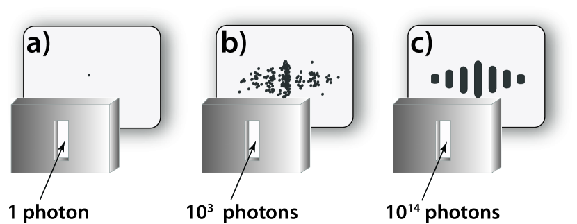
Figure 1: Interference effect in the single slit experiment for a) 1 , b) $10^{3}$, and c) $10^{14}$ photons or particles.

The new paradigm in physics which emerged at the beginning of the last century and is now commonly referred to as quantum mechanics was motivated by two kinds of experimental observations: the “lumpiness”, or quantization, of energy transfer in light-matter interactions, and the dual wave-particle nature of both light and matter. Max Planck could correctly calculate the spectrum of black-body radiation in 1900 by postulating that an electromagnetic field can exchange energy with atoms only in quanta which are the product of the radiation frequency and the famous constant $h$, which was later named after him planck . Whereas for Planck himself, the introduction of his constant was an act of desperation, solely justified by the agreement of the calculated with the measured spectrum, Albert Einstein took the idea serious. In his explanation of the photoelectric effect in 1905, he considered light itself as being composed of particles carrying a discrete energy einstein . This bold view was in blatant contradiction with the by then established notion of light as an electromagnetic wave. The latter belief was supported, for instance, by the observation of interference: If we shine light on a single slit placed in front of a scintillating screen, we observe a pattern of darker and brighter fringes or rings. But what happens if Einstein’s light particles, let us call them photons, exist and we zing them one-by-one at the same slit? Then, each photon causes the screen to scintillate only at a single point. However, after a large number of photons pass through the slit one at a time, we once again obtain an interference pattern. This build-up of interference one photon at a time is illustrated in Fig. 1.

In 1913, Niels Bohr succeeded in deriving the discrete lines of the hydrogen spectrum with a simple atomic model in which the electron circles the proton just as a planet orbits the sun, supplemented by the ad-hoc assumption that the orbital angular momentum must be an integer multiple of $\hbar=h/2\pi$, which leads to discrete energies of the corresponding orbitals bohr . Further, transitions between these energy levels are accompanied by the absorption or emission of a photon whose frequency is $E/h$, where $E$ is the energy difference of the two levels. Apparently, the quantization of light is strongly tied to the quantization within matter. Inspired by his predecessors, Louis de Broglie suggested that not only light has particle characteristics, but that classical particles, such as electrons, have wave characteristics broglie . He associated the wavelength $\lambda$ of these waves with the particle momentum $p$ through the relation $p=h/\lambda$. Interestingly, Bohr’s condition for the orbital momentum of the electron is equivalent with the demand that the length of an orbital path of the electron has to be an integer multiple of its de Broglie wavelength.

Erwin Schrödinger was very intrigued by de Broglie’s ideas and set his mind on finding a wave equation for the electron. Closely following the electromagnetic prototype of a wave equation, and attempting to describe the electron relativistically, he first arrived at what we today know as the Klein-Gordon-equation. To his annoyance, however, this equation, when applied to the hydrogen atom, did not result in energy levels consistent with Arnold Sommerfeld’s fine structure formula, a refinement of the energy levels according to Bohr. Schrödinger therefore retreated to the non-relativistic case, and obtained as the non-relativistic limit to his original equation the famous equation that now bears his name. He published his results in a series of four papers in 1926 schroedinger1 ; schroedinger2 ; schroedinger3 ; schroedinger4 . Therein, he emphasizes the analogy between electrodynamics as a wave theory of light, which in the limit of small electromagnetic wavelength approaches ray optics, and his wave theory of matter, which approaches classical mechanics in the limit of small de Broglie wavelengths. His theory was consequently called wave mechanics. In a wave mechanical treatment of the hydrogen atom and other bound particle systems, the quantization of energy levels followed naturally from the boundary conditions. A year earlier, Werner Heisenberg had developed his matrix mechanics heisenberg , which yielded the values of all measurable physical quantities as eigenvalues of a matrix. Schrödinger succeeded in showing the mathematical equivalence of matrix and wave mechanics schroedinger5 ; they are just two different descriptions of quantum mechanics. A relativistic equation for the electron was found by Paul Dirac in 1927 dirac . It included the electron spin of $1/2$, a purely quantum mechanical feature without classical analog. Schrödinger’s original equation was taken up by Klein and Gordon, and eventually turned out to be a relativistic equation for bosons, i.e. particles with integer spin. In spite of its limitation to non-relativistic particles, and initial rejection from Heisenberg and colleagues, the Schrödinger equation became eventually very popular. Today, it provides the material for a large fraction of most introductory quantum mechanics courses.

III The Schrödinger equation derived

Our approach to the Schrödinger equation will be similar to that taken by Schrödinger himself. We start with the classical wave equation, as derived from Maxwell’s equations governing classical electrodynamics (see the appendix). For simplicity, we consider only one dimension,

$$\frac{\partial^{2}E}{\partial^{2}x}-\frac{1}{c^{2}}\frac{\partial^{2}E}{\partial^{2}t}=0.$$ (1)

This equation is satisfied by plane wave solutions,

$$E(x,t)=E_{0}e^{i(kx-\omega t)},$$ (2)

where $k=2\pi/\lambda$ and $\omega=2\pi\nu$ are the spatial and temporal frequencies, respectively, which must satisfy the dispersion relation obtained upon substitution of Eq. (2) into Eq. (1):

$$\left(\frac{\partial^{2}}{\partial^{2}x}-\frac{1}{c^{2}}\frac{\partial^{2}}{\partial^{2}t}\right)E_{0}e^{i(kx-\omega t)} = 0,$$ (3)

$$\left(-k^{2}+\frac{\omega^{2}}{c^{2}}\right)E_{0}e^{i(kx-\omega t)} = 0.$$ (4)

Solving for the wave vector, we arrive at the dispersion relation for light in free space:

$$k=\frac{\omega}{c},$$ (5)

or more familiarly

$$\nu\lambda=c,$$ (6)

where $c$ is the wave propagation speed, in this case the speed of light in vacuum. These solutions represent classical electromagnetic waves, which we know are somehow related to the quantum theory’s photons.

Recall from Einstein and Compton that the energy of a photon is $\mathcal{E}=h\nu=\hbar\omega$ and the momentum of a photon is $p=h/\lambda=\hbar k$. We can rewrite Eq. (2) using these relations:

$$E(x,t)=E_{0}e^{\frac{i}{\hbar}(px-\mathcal{E}t)}.$$ (7)

Substituting this into Eq. (1), we find

$$\left(\frac{\partial^{2}}{\partial^{2}x}-\frac{1}{c^{2}}\frac{\partial^{2}}{\partial^{2}t}\right)E_{0}e^{\frac{i}{\hbar}(px-\mathcal{E}t)} = 0,$$ (8)

$$-\frac{1}{\hbar^{2}}\left(p^{2}-\frac{\mathcal{E}^{2}}{c^{2}}\right)E_{0}e^{\frac{i}{\hbar}(px-\mathcal{E}t)} = 0,$$ (9)

or

$$\mathcal{E}^{2}=p^{2}c^{2}.$$ (10)

This is just the relativistic total energy,

$$\mathcal{E}^{2}=p^{2}c^{2}+m^{2}c^{4},$$ (11)

for a particle with zero rest mass, which is reassuring since light is made of photons, and photons travel at the speed of light in vacuum, which is only possible for particles of zero rest mass.

We now assume with de Broglie that frequency and energy, and wavelength and momentum, are related in the same way for classical particles as for photons, and consider a wave equation for non-zero rest mass particles. That means, we want to end up with $\mathcal{E}^{2}=p^{2}c^{2}+m^{2}c^{4}$ instead of just $\mathcal{E}^{2}=p^{2}c^{2}$. Since we do not deal with an electric field any more, we give the solution to our wave equation a new name, say $\Psi$, and simply call it the wave function. In doing so, we have exploited that Eq. (8) is homogenous, and hence the units of the function operated upon are arbitrary. Instead of Eq. (9), we would now like

$$-\frac{1}{\hbar^{2}}\left(p^{2}-\frac{\mathcal{E}^{2}}{c^{2}}+m^{2}c^{2}\right)\Psi\,e^{\frac{i}{\hbar}(px-\mathcal{E}t)}=0,$$ (12)

which we can get from

$$\left(\frac{\partial^{2}}{\partial^{2}x}-\frac{1}{c^{2}}\frac{\partial^{2}}{\partial^{2}t}-\frac{m^{2}c^{2}}{\hbar^{2}}\ \right)\Psi\,e^{\frac{i}{\hbar}(px-\mathcal{E}t)}=0.$$ (13)

In the discussion of light as a wave or a collection of photons, it turns out that the square of the electric field is proportional to the number of photons. By anology, we demand that our wave function,

$$\Psi(x,t)=\Psi_{0}e^{\frac{i}{\hbar}(px-\mathcal{E}t)},$$ (14)

be normalizable to unit probability. Then, the probability that the particle is located somewhere in space,

$$\int_{-\infty}^{\infty}\Psi^{*}\Psi d\,x=1,$$ (15)

as it should be.

Removing restriction to one dimension and rearranging, we recognize this as the Klein-Gordon equation for a free particle,

$$\nabla^{2}\Psi-\frac{m^{2}c^{2}}{\hbar^{2}}\Psi=\frac{1}{c^{2}}\frac{\partial^{2}\Psi}{\partial^{2}t}.$$ (16)

The Klein-Gordon equation is a relativistic equation, the Schrödinger equation is not. So to ultimately arrive at the Schrödinger equation, we must make the assumptions necessary to establish a non-relativistic equation.

The first step in considering the non-relativistic case is to approximate $\mathcal{E}^{2}=p^{2}c^{2}+m^{2}c^{4}$ as follows:

$$\mathcal{E} = mc^{2}\sqrt{1+\frac{p^{2}}{m^{2}c^{2}}},$$ (17)

$$\approx mc^{2}\left(1+\frac{1}{2}\frac{p^{2}}{m^{2}c^{2}}\right),$$ (18)

$$\approx mc^{2}+\frac{p^{2}}{2m}=mc^{2}+\mathcal{T}.$$ (19)

We recognize this last term as the classical kinetic energy, $\mathcal{T}$. We can then rewrite the wave equation, Eq. (14), as

$$\Psi(x,t) = \Psi_{0}e^{\frac{i}{\hbar}(px-mc^{2}t-\mathcal{T}t)},$$ (20)

$$= e^{-\frac{i}{\hbar}mc^{2}t}\Psi_{0}e^{\frac{i}{\hbar}(px-\mathcal{T}t)}.$$ (21)

We have assumed that the particle velocity is small such that $mv\ll mc$, which implies that $p^{2}\ll m^{2}c^{2}$. This means that the leading term in Eq. (21), $\exp(-imc^{2}t/\hbar)$, will oscillate much faster than the last term, $\exp(i\mathcal{T}t/\hbar)$. Taking advantage of this, we can write

$$\Psi=e^{-\frac{i}{\hbar}mc^{2}t}\phi,$$ (22)

where

$$\phi=\Psi_{0}e^{\frac{i}{\hbar}(px-\mathcal{T}t)}.$$ (23)

Then

$$\frac{\partial\Psi}{\partial\,t} = -\frac{i}{\hbar}mc^{2}e^{-\frac{i}{\hbar}mc^{2}t}\phi+e^{\frac{-i}{\hbar}mc^{2}t}\frac{\partial\phi}{\partial\,t}$$ (24)

$$\frac{\partial^{2}\Psi}{\partial\,t^{2}} = \Bigl{(}-\frac{m^{2}c^{4}}{\hbar^{2}}e^{-\frac{i}{\hbar}mc^{2}t}\phi-\frac{2i}{\hbar}mc^{2}e^{-\frac{i}{\hbar}mc^{2}t}\frac{\partial\phi}{\partial\,t}\Bigl{)}+e^{-\frac{i}{\hbar}mc^{2}t}\frac{\partial^{2}\phi}{\partial\,t^{2}}.$$ (25)

The first term in brackets is large and the last term is small. We keep the large terms and discard the small one. Using this approximation in the Klein-Gordon equation, Eq. (13), we find

$$e^{-\frac{i}{\hbar}mc^{2}t}\Bigl{[}\frac{\partial^{2}}{\partial\,x^{2}}+\frac{2im}{\hbar}\frac{\partial}{\partial\,t}\Bigl{]}\phi = 0,$$ (26)

$$\frac{\partial^{2}\phi}{\partial\,x^{2}}+\frac{2im}{\hbar}\frac{\partial\phi}{\partial\,t} = 0.$$ (27)

Again rearranging and generalizing to three spatial dimensions, we finally arrive at the Schrödinger equation for a free particle (zero potential):

$$-\frac{\hbar^{2}}{2m}\nabla^{2}\phi=i\hbar\frac{\partial\phi}{\partial t},$$ (28)

where the non-relativistic wave function $\phi$ is also constrained to the condition that it be normalizable to unit probability.

IV Conclusion

The simple derivation of the Schrödinger equation provided here requires only basic knowledge of the electromagnetic scalar wave equation and the basics of Einstein’s special theory of relativity. Both of these topics, and the approximations used in our derivation, are commonly covered prior to a first course in quantum mechanics. Taking the approach that we have outlined exposes students to the reasoning employed by the founders themselves. Though much has been done to refine our understanding of quantum mechanics, taking a step back and thinking through the problem the way they did has merit if our goal as educators is to produce the next generation of Schrödingers.

We have glossed over the statistical interpretation of quantum mechanics, which is dealt with superbly in any number of the standard textbooks, and particularly well in Griffiths’ text griffiths . We have also considered only single particles. Many independent particles are a trivial extension of what we have shown here, but in the presence of interparticle coupling, quantum statistical mechanics is a distraction we can do without, given the narrow objective outlined in the title of this paper. Spin, which is relevant for a fully relativistic treatment of the electron or when more than one particle is considered, has also not been discussed. An obvious next step would be to consider a particle in a potential, but we believe that doing so would result in diminishing returns due to the added complications a potential introduces. What we have shown here is the missing content for the lecture on day one in an introductory quantum mechanics course. Spin, interparticle coupling, and potentials are already adequately covered elsewhere.

Appendix A The Electromagnetic Wave Equation

The wave equation governing electromagnetic waves in free space is derived from Maxwell’s equations in free space, which are:

$$\nabla\times\mathbf{E} = -\frac{\partial\mathbf{B}}{\partial\,t},$$ (29)

$$\nabla\times\mathbf{B} = \frac{1}{c^{2}}\frac{\partial\mathbf{E}}{\partial\,t},$$ (30)

$$\nabla\cdot\mathbf{E} = 0,$$ (31)

$$\nabla\cdot\mathbf{B} = 0,$$ (32)

where $c$ is the speed of light in vacuum, $\mathbf{E}$ is the electric field, and $\mathbf{B}$ is the magnetic field. The first equation embodies Faraday’s law and illustrates the generation of a voltage by a changing magnetic field. This equation is the basis of electric generators, inductors, and transformers. The second equation embodies Ampere’s law and is the magnetic analogy of the first equation. It explains, for example, why there is a circulating magnetic field surrounding a wire with electrical current running through it. It is the basis of electromagnets and the magnetic poles associated with the rotating ion core in the earth. The last two equations are embodiments of Gauss’ law for electricity and for magnetism, respectively. In the case of electricity, it is consistent with Coulomb’s law and stipulates that charge is a source for the electric field. If charges are present, then the right-hand side of Eq. (31) is non-zero and proportional to the charge density. The magnetic case is often referred to as the “no magnetic monopoles” law. Since there are no magnetic monopoles (intrinsic magnetic charge carriers), Eq. (32) always holds.

Applying the curl operator to both sides of Eq. (29) and substituting $\nabla\times\mathbf{B}$ from Eq. (30), we find:

$$\nabla\times(\nabla\times\mathbf{E})=-\frac{1}{c^{2}}\frac{\partial^{2}\mathbf{E}}{\partial^{2}t}.$$ (33)

Next, we apply the familiar vector identityjackson , $\nabla\times(\nabla\times\Box)=\nabla(\nabla\cdot\Box)-\nabla^{2}\Box$, where $\Box$ is any vector, to the left hand side of Eq. (33):

$$\nabla\times(\nabla\times\mathbf{E})=\nabla(\nabla\cdot\mathbf{E})-\nabla^{2}\mathbf{E}.$$ (34)

From Eq. (31), this reduces to:

$$\nabla^{2}\mathbf{E}-\frac{1}{c^{2}}\frac{\partial^{2}\mathbf{E}}{\partial^{2}t}=0,$$ (35)

which is the electromagnetic wave equation.

- (1) D.J. Griffiths, Introduction to Quantum Mechanics, (Prentice Hall, New Jersey, 2005), 2nd ed.
- (2) E. Merzbacher, Quantum Mechanics, (Wiley, New York, 1998), 3rd ed.
- (3) J.J. Sakurai, Modern Quantum Mechanics, (Addison-Wesley, Massachusetts, 1994), Rev. ed.
- (4) M.J.W. Hall, M. Reginatto, “Schrödinger equation from an exact uncertainty principle,” J. Phys. A 35, 3289-3303 (2002).
- (5) P. Peice, “Another Schrödinger derivation of the equation,” Eur. J. Phys. 17,116 117 (1996).
- (6) J.H. Field, “Relationship of quantum mechanics to classical electromagnetism and classical relativistic mechanics,” Eur. J. Phys. 25, 385-397 (2004).
- (7) J. Ogborn and E.F. Taylor, “Quantum physics explains Newton’s laws of motion,” Phys. Educ. 40, (1), 26-34 (2005).
- (8) E. Nelson, “Derivation of the Schrödinger equation from Newtonian mechanics,” Phys. Rev. 150, (4), 1079-1085 (1966).
- (9) J. Bernstein, “Max Born and the quantum theory,” Am. J. Phys. 73, (11), 999-1008 (2005).
- (10) M. Planck, “Über das Gesetz der Energieverteilung im Normalspektrum / On the law of distribution of energy in the normal spectrum,” Annalen der Physik 309 (4th series 4), (3), 553-563 (1901).
- (11) A. Einstein, “Über einen die Erzeugung und Verwandlung des Lichtes betreffenden heuristischen Gesichtspunkt / On a heuristic viewpoint concerning the production and transformation of light,” Annalen der Physik 322 (4th series 17), (6), 132-148 (1905).
- (12) N. Bohr, “On the constitution of atoms and molecules,” Philosophical Magazin 26, (6), 1-25 (1913).
- (13) L. de Broglie, “Recherches sur la theorie des quanta / On the theory of quanta,” Annales de Physique 3, 22 (1925).
- (14) E. Schrödinger, “Quantisierung als Eigenwertproblem. (Erste Mitteilung.) / Quantisation as an eigenvalue problem. (First Communication.),” Annalen der Physik 384, (4), 361-376 (1926).
- (15) E. Schrödinger, “Quantisierung als Eigenwertproblem. (Zweite Mitteilung.) / Quantisation as an eigenvalue problem. (Second Communication.),” Annalen der Physik 384, (6), 489-527 (1926).
- (16) E. Schrödinger, “Quantisierung als Eigenwertproblem. (Dritte Mitteilung.) / Quantisation as an eigenvalue problem. (Third Communication.),” Annalen der Physik 385, (13), 437-490 (1926).
- (17) E. Schrödinger, “Quantisierung als Eigenwertproblem. (Vierte Mitteilung.) / Quantisation as an eigenvalue problem. (Fourth Communication.),” Annalen der Physik 386, (18), 109-139 (1926).
- (18) W. Heisenberg, “Über die quantentheoretische Umdeutung kinematischer und mechanischer Beziehungen / On the quantum theoretical re-interpretation of kinematic and mechanical relations,” Zeitschrift für Physik 33, 879 (1925).
- (19) E. Schrödinger, “Über das Verhaeltnis der Heisenberg-Born-Jordanschen Quantenmechanik zu der meinen / On the relationship of the Heisenberg-Born-Jordan quantum mechanics to mine,” Annalen der Physik 384, (8), 734-756 (1926).
- (20) P. Dirac, “The quantum theory of the electron,” Proc. Roy. Soc. A 117, 610-624 (1928).
- (21) J.D. Jackson, Classical Electrodynamics, (Wiley, New York, 1999), 3rd ed.