Self-organization of the Sound Inventories: Analysis and Synthesis of the Occurrence and Co-occurrence Networks of Consonants

Abstract

The sound inventories of the world’s languages self-organize themselves giving rise to similar cross-linguistic patterns. In this work we attempt to capture this phenomenon of self-organization, which shapes the structure of the consonant inventories, through a complex network approach. For this purpose we define the occurrence and co-occurrence networks of consonants and systematically study some of their important topological properties. A crucial observation is that the occurrence as well as the co-occurrence of consonants across languages follow a power law distribution. This property is arguably a consequence of the principle of preferential attachment. In order to support this argument we propose a synthesis model which reproduces the degree distribution for the networks to a close approximation. We further observe that the co-occurrence network of consonants show a high degree of clustering and subsequently refine our synthesis model in order to incorporate this property. Finally, we discuss how preferential attachment manifests itself through the evolutionary nature of language.

1 Introduction

Sound inventories of human languages show a considerable extent of symmetry. This symmetry is primarily a reflection of the self-organizing behavior that goes on in shaping the structure of the inventories (?, ?). It has been postulated previously that such a self-organizing behavior can be explained through the principles of functional phonology, namely, maximal perceptual contrast (?, ?), ease of articulation (?, ?, ?), and ease of learnability (?, ?). These explanations are an outcome of the macroscopic level (?, ?) of analysis, and are quite commonly used by traditional linguists (?, ?, ?, ?, ?, ?). Of late, it has been shown that even in the microscopic level (?, ?), the emergent behavior of the vowel inventories in particular, can be satisfactorily explained through multi-agent simulation models (?, ?). However, instances of such modeling either in the micro or in the mesoscopic levels (?, ?) to demonstrate the organizational principles of the consonant inventories, are absent in literature.

In this work we present a mesoscopic model, grounded on the theories of complex networks (for a review see (?, ?, ?)), in order to capture the self-organizing principles of the consonant inventories. We call our model mesoscopic since it does not make use of the functional properties of the macro level for explaining the structure of the consonant inventories; nor does it incorporate microscopic interactions between the speakers of a language (usually modeled through linguistic agents (?, ?)), in order to reproduce this structure. We rather base our model on slightly coarse grained components like languages and consonants, and study the interactions between and within them respectively. In order to capture these interactions we define two networks namely, PlaNet or the Phoneme Language Network and PhoNet or the Phoneme Phoneme Network. PlaNet is a bipartite network which has two sets of nodes, one labeled by the languages while the other by the consonants. Edges run between the nodes of these two sets depending on whether or not a particular consonant occurs in a particular language. On the other hand, PhoNet is the one-mode projection of PlaNet onto the consonant nodes. Hence PhoNet is a weighted unipartite network of consonants where an edge between two nodes signifies their co-occurrence likelihood over the consonant inventories. The construction of PlaNet, and subsequently PhoNet, are motivated by similar modeling of various complex phenomena observed in nature and society, such as,

• Movie-actor network, where movies and actors constitute the two partitions and an edge between them signifies that a particular actor acted in a particular movie (?, ?). In the corresponding one-mode projection onto the actor nodes, any two actors are connected as many times as they have co-acted in a movie.

• Article-author network, where the edges denote which person has authored which articles (?, ?). In this case the one-mode projection onto the author nodes comprises of a pair of authors connected as many times as they have co-authored an article.

• Metabolic network of organisms, where the corresponding partitions are chemical compounds and metabolic reactions. Edges run between partitions depending on whether a particular compound is a substrate or result of a reaction (?, ?). In this case the one-mode projection onto the chemical compounds comprises a pair of compounds connected by as many edges as they have co-participated in a metabolic reaction.

Modeling of the complex systems referred above as networks has proved to be a comprehensive and emerging way of capturing the underlying generating mechanisms of such systems (?, ?, ?). In this direction there have been some attempts as well to model the intricacies of human languages through complex networks. Word networks based on synonymy (?, ?), co-occurrence (?, ?), and phonemic edit-distance (?, ?) are examples of such attempts. The present work also uses the concept of complex networks to develop a platform for a holistic analysis as well as synthesis of the distribution of the consonants across the languages.

In the current work we present some of the exciting properties of the consonant inventories through the analysis as well as synthesis of PlaNet and PhoNet. A significant property we observe is that the consonant nodes in PlaNet as well as PhoNet have a power law degree distribution with an exponential cut-off. This property is arguably a consequence of the principle of preferential attachment (?, ?). In order to support this argument we present a synthesis model for PlaNet which generates the degree distribution of the consonant nodes and mimics the real data to a very close approximation. However, though the degree distributions of the empirical and the synthesized PlaNet match closely, their one-mode projections (the empirical and the synthesized PhoNet) seem to differ especially in their clustering coefficients (?, ?). The clustering coefficient of the empirical PhoNet is substantially higher than that of the synthesized version, indicating that consonants tend to frequently occur in cohesive groups or communities (?, ?). We therefore modify the synthesis model and allow triad (i.e., fully connected triplets) formation. As a consequence of this modification the degree distributions of PlaNet and PhoNet as well as the clustering coefficient of PhoNet match their respective synthesized versions with a very high accuracy.

The rest of the article is structured as follows. In section 2 we formally define PlaNet and PhoNet and outline their construction procedure. We also present some interesting studies pertaining to the structural properties of PlaNet as well as PhoNet in the same section. In section 3 we propose a synthesis model for PlaNet based on the principle of preferential attachment. We also identify some necessary refinements in the synthesis model (in order to improve upon the average clustering coefficient of PhoNet) and subsequently extend it to incorporate these refinements in the same section. Finally we conclude in section 4 by summarizing our contributions, pointing out some of the implications of the current work and indicating the possible future directions.

2 Definition, Construction and Analysis of PlaNet and PhoNet

In this section we formally define PlaNet and PhoNet followed by a description of their construction procedure. We also present some interesting studies pertaining to the topological properties of these networks.

2.1 Definition

Definition of PlaNet: We define PlaNet (the network of consonants and languages) as a bipartite graph G = $\langle$V_L, V_C, E$\rangle$ where V_L is the set of nodes labeled by the languages and V_C is the set of nodes labeled by the consonants. E is the set of edges that run between V_L and V_C. There is an edge $e$ $\in$ E between two nodes $v_{l}$ $\in$ V_L and $v_{c}$ $\in$ V_C if and only if the consonant c occurs in the language l. Figure 1 illustrates the nodes and edges of PlaNet.

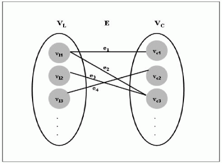
Figure 1: Illustration of the nodes and edges of PlaNet.

Definition of PhoNet: PhoNet, which is the one-mode projection of PlaNet (projection taken on the consonant nodes), can be defined as a network of consonants represented by a graph G = $\langle$ V_C, E $\rangle$ where V_C is the set of nodes labeled by the consonants and E is the set of all the edges in G. There is an edge $e$ $\in$ E between two nodes, if and only if there exists one or more language(s) where the nodes (read consonants) co-occur. The weight of the edge $e$ (also edge-weight) is the number of languages in which the consonants connected by $e$ co-occur. Figure 2 presents a partial illustration of PhoNet.

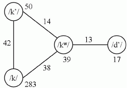
Figure 2: A partial illustration of the nodes and edges in PhoNet. The labels of the nodes denote the consonants represented in IPA (International Phonetic Alphabet). The numerical values against the edges and nodes represent their corresponding weights. For example /$k$/ occurs in 283 languages; /$k^{w}$/ occurs in 39 languages while they co-occur in 38 languages.

2.2 Construction

Construction of PlaNet: Many typological studies (?, ?, ?, ?) of segmental inventories have been carried out in past on the UCLA Phonological Segment Inventory Database (UPSID) (?, ?). UPSID records the sound inventories of 317 languages covering all the major language families of the world. In this work we have used UPSID comprising of these 317 languages and 541 consonants found across them, for constructing PlaNet. Consequently, there are 317 elements (nodes) in the set V_L and 541 elements (nodes) in the set V_C. The number of elements (edges) in the set E as computed from PlaNet is 7022. At this point it is important to mention that in order to avoid any confusion in the construction of PlaNet we have appropriately filtered out the anomalous and the ambiguous segments (?, ?) from it. In UPSID, a segment has been classified as anomalous if its existence is doubtful and ambiguous if there is insufficient information about the segment. For example, the presence of both the palatalized dental plosive and the palatalized alveolar plosive are represented in UPSID as palatalized dental-alveolar plosive. According to popular techniques (?, ?), we have completely ignored the anomalous segments from the data set, and included the ambiguous ones as separate segments because there are no descriptive sources explaining how such ambiguities might be resolved.

Construction of PhoNet: Once PlaNet is constructed as described above, we can easily construct PhoNet by taking an one-mode projection of PlaNet onto the consonant nodes. Consequently, the set V_C for PhoNet comprises of 541 elements (nodes) and the set E comprises of 34012 elements (edges).

2.3 Degree Distribution

The degree of a node $u$, denoted by $k_{u}$ is defined as the number of edges connected to $u$. The term degree distribution is used to denote the way degrees ($k_{u}$) are distributed over the nodes ($u$).

2.3.1 Degree Distribution of PlaNet

Since PlaNet is bipartite in nature it has two degree distribution curves one corresponding to the nodes in the set V_L and the other corresponding to the nodes in the set V_C.

Degree distribution of the nodes in V_L: Figure 3 shows the degree distribution of the nodes in V_L where the x-axis denotes the degree of each node expressed as a fraction of the maximum degree and the y-axis denotes the number of nodes having a given degree expressed as a fraction of the total number of nodes in V_L.

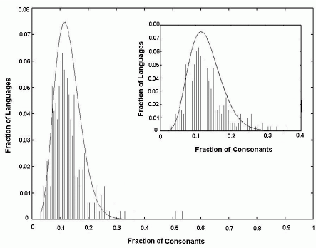
Figure 3: Degree distribution of PlaNet for the set V_L. The figure in the inner box is a magnified version of a portion of the original figure.

Figure 3 indicates that the number of consonants appearing in different languages follow a $\beta$-distribution (see (?, ?) for reference) which is right skewed with the values of $\alpha$ and $\beta$ equal to 7.06 and 47.64 (obtained using maximum likelihood estimation method) respectively. This asymmetry in the distribution points to the fact that languages usually tend to have smaller consonant inventory size, the best value being somewhere between 10 and 30. The distribution peaks roughly at 21 (which is its mode) whereas the mean of the distribution is 22 indicating that on an average the languages in UPSID have a consonant inventory of 22 (?, ?).

Degree distribution of the nodes in V_C: Figure 4 illustrates the degree distribution plot for the nodes in V_C in log-log scale. In this figure the x-axis represents the degree ($k$) and the y-axis represents $P_{k}$, where $P_{k}$ is the fraction of nodes having degree greater than or equal to $k$.

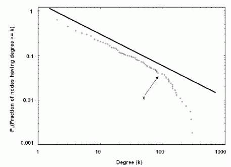
Figure 4: Degree distribution of PlaNet for the set V_C in a log-log scale. The letter x denotes the cut-off point.

Figure 4 clearly shows that the curve follows a power law distribution with an exponential cut-off. The cut-off point is indicated by the letter x in the figure. We find that there are 22 consonant nodes which have their degree above the cut-off range. However, the remaining consonant nodes of PlaNet exhibit a power law degree distribution of the form

$$y=Ax^{-\gamma}$$ (1)

The values of the parameters A and $\gamma$ in both the figures, as computed by the least square error method, are noted in Table 1.

Table 1: The values of the parameters A and $\gamma$.

Parameter	Figure 4	Figure 5
A	1.04	41.26
$\gamma$	0.71	0.89

2.3.2 Degree Distribution of PhoNet

Since PhoNet is a weighted network, we report the distribution of the weighted degree of its nodes. The weighted degree $k$ for a node $i$ can be defined as (?, ?),

$$k=\sum_{\forall j}w_{ij}$$ (2)

where $j$ is a neighbor of $i$ in the network and $w_{ij}$ is the weight of the edge connecting the nodes $i$ and $j$. Figure 5 shows the degree distribution curve for PhoNet in log-log scale. In this figure the x-axis represents the weighted degree ($k$) and the y-axis represents $P_{k}$, where $P_{k}$ is the fraction of nodes having degree greater than or equal to $k$. Interestingly, the degree distribution of the nodes in PhoNet show two different cut-off points marked by the letters x and y in the figure along with a power law region spanning from x to y. Through inspection we find that there are 15 consonants above the cut-off x which indicates that these consonants co-occur very frequently exhibiting an hub-like nature (?, ?, ?). On the other hand, the degree distribution of the nodes up to the cut-off point y is approximately a straight line indicating that the rate of change of $P_{k}$ with respect to $k$ is quite slow in this region. The reason behind this behavior is that there are only a negligibly small fraction of nodes that exist in this region which, causes almost no increase in the cumulative fraction $P_{k}$. However, the rest of the consonant nodes (spanning from the point y to the point x) show a power law degree distribution of the form specified in equation 1. Table 1 reports the values of the parameters A and $\gamma$.

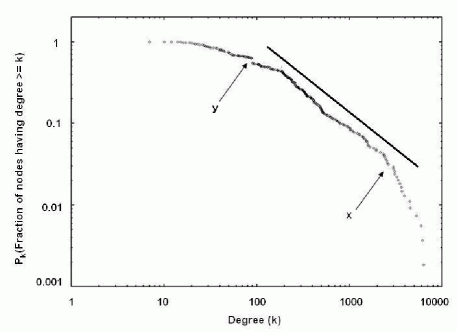
Figure 5: Degree distribution of the nodes in PhoNet in a log-log scale. The letters x and y denote the cut-off points.

In most of the networked systems like the society, the Internet, the World Wide Web, and many others, power law degree distribution emerges for the phenomenon of preferential attachment, i.e., when “the rich get richer” (?, ?). With reference to PlaNet and PhoNet this preferential attachment can be interpreted as the tendency of a language to choose a consonant that has been already chosen by a large number of other languages. In order to validate the above argument, in section 3, we present a synthesis model based on preferential attachment (where the distribution of the consonant inventory size is known a priori) that mimics the occurrence and co-occurrence distributions of the consonant nodes to a very close approximation.

2.4 Clustering Coefficient

The weighted clustering coefficient (in the one-mode projection PhoNet) for a node $i$ is defined as (?, ?),

$$c_{i}=\frac{1}{\left(\sum_{\forall j}w_{ij}\right)(k_{i}-1)}{\sum_{\forall j,l}\frac{(w_{ij}+w_{il})}{2}a_{ij}a_{il}a_{jl}}$$ (3)

where $j$ and $l$ are neighbors of $i$; $k_{i}$ represents the plain degree of the node $i$; $w_{ij}$, $w_{jl}$ and $w_{il}$ denote the weights of the edges connecting nodes $i$ and $j$, $j$ and $l$, and $i$ and $l$ respectively; $a_{ij}$, $a_{il}$, $a_{jl}$ are boolean variables indicating whether or not there is an edge between the nodes $i$ and $j$, $i$ and $l$, and $j$ and $l$ respectively. This coefficient is a measure of the local cohesiveness that takes into account the importance of the clustered structure on the basis of the amount of traffic or interaction intensity actually found on the local triplets. The parameter $c_{i}$ in equation 3 counts for each triplet formed in the neighborhood of the vertex $i$, the weight of the two participating edges of the vertex $i$. The normalization factor $\left(\sum_{\forall j}w_{ij}\right)(k_{i}-1)$ accounts for the weight of each edge times the maximum possible number of triplets in which it may participate, and it ensures that $0~{}\leq~{}c_{i}~{}\leq~{}1$. Consequently, the average weighted clustering coefficient is given by,

$$c_{av}=\frac{1}{N}{\sum_{i=1}^{N}c_{i}}$$ (4)

where, $N$ is the number of nodes in PhoNet.

The value of $c_{av}$ for PhoNet is 0.89 which indicates a huge clustering among the nodes of the network. This is primarily due to the fact that in PhoNet the consonant nodes tend to occur highly in cohesive groups or communities as shown by Mukherjee et al. (?, ?). In order to further investigate how the clustering coefficient is related to the weighted degree of the nodes of PhoNet we plot the degree-dependent clusterings in Figure 6 in log-log scale. The figure shows a scatter plot as well as an average binned distribution with bin sizes expressed as powers of 2. It is quite interesting to observe that like many other social networks (?, ?) in this case also the clustering is substantial (very close to one) for vertices with small degrees and gets lower with an increasing $k$. This is because the more neighbors a consonant node has the less probable it will be for those neighbors to co-occur in the same language and hence be connected with each other.

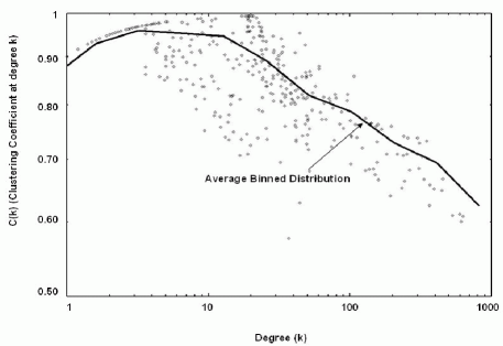
Figure 6: Degree versus clustering coefficient for the nodes of PhoNet in log-log scale. The bold line shows the average binned distribution with bin sizes expressed in powers of 2.

The power law degree distributions observed for both PlaNet and PhoNet are indicative of the presence of preferential attachment in the organization of the consonant inventories. We are however interested in estimating the amount of preferential attachment involved to get an accurate view of the underlying dynamics guiding the formation of the consonant inventories. This can be best understood through a synthesis model which, we present in the next section that mimics the empirical data to a high precision.

3 Synthesis Model Based on Preferential Attachment

In this section we present a synthesis model for the PlaNet (henceforth PlaNet_syn) based on preferential attachment where the distribution of the consonant inventory size is assumed to be known a priori. Let V_L = {L₁,L₂,…,L₃₁₇} have cardinalities (consonant inventory size) {k₁,k₂,…,k₃₁₇} respectively. We assume that the consonant nodes (V_C) of PlaNet_syn are unlabeled (i.e., they are not labeled by a set of articulatory/acoustic features (?, ?) that characterizes them). We next sort the nodes L₁ through L₃₁₇ in ascending order of their cardinalities. At each time step a node L_j, chosen in order, preferentially attaches itself with k_j distinct nodes (call each such node C_i) of the set V_C. The probability $Pr(C_{i})$ with which the node L_j attaches itself to the node C_i is given by,

$$Pr(C_{i})=\frac{{d_{i}}^{\alpha}+\epsilon}{\sum_{{i^{{}^{\prime}}}\in V^{{}^{\prime}}_{C}}({d_{i^{{}^{\prime}}}}^{\alpha}+\epsilon)}$$ (5)

where, $d_{i}$ is the current degree of the node $C_{i}$, V${}^{{}^{\prime}}_{C}$ is the set of nodes in V_C that are not already connected to L_j and $\epsilon$ is the smoothing parameter which facilitates attachments to consonant nodes that have a degree close or equal to zero. The above process is repeated until all the language nodes L${}_{j}\in$V_L get connected to k_j consonant nodes. Algorithm 1 summarizes the synthesis process and Figure 7 illustrates a partial step of this process.

Algorithm 1: The synthesis process
Input: Nodes L1 through L317 sorted in ascending
order of their cardinalities;
for $t$ = 1 to 317 {
Choose (in order) a node Lj with cardinality kj;
for $c$ = 1 to kj {
Connect Lj to a node Ci $\in$ VC to which it is
not yet connected, following the distribution,
$Pr(C_{i})=\frac{{d_{i}}^{\alpha}+\epsilon}{\sum_{{i^{{}^{\prime}}}\in V^{{}^{\prime}}_{C}}({d_{i^{{}^{\prime}}}}^{\alpha}+\epsilon)}$
where V${}^{{}^{\prime}}_{C}$ is the set of nodes in VC to which
Lj is not yet connected;
}
}

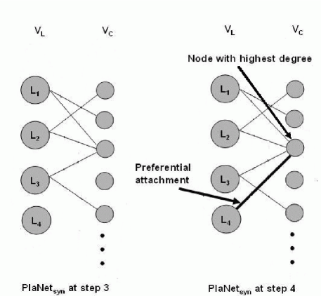
Figure 7: A partial step of the synthesis process. When the language L₄ has to connect itself with one of the nodes in the set V_C it does so with the one having the highest degree (=3) rather than with others in order to achieve preferential attachment which is the working principle of our algorithm.

As we shall see shortly, the aforementioned preferential attachment based model is able to explain the distribution of the consonants over languages reasonably well. However, at this point it would be worthwhile to mention the reason behind sorting the language nodes in ascending order of their cardinalities. With each consonant is associated two different frequencies; a) the frequency of occurrence of a consonant over languages or the type frequency, and b) the frequency of usage of the consonant in a particular language or the token frequency. Researchers have shown in the past that these two frequencies are positively correlated. Nevertheless, our synthesis model based on preferential attachment takes into account only the type frequency of a consonant and not its token frequency. If language is considered to be an evolving system (?, ?) then both of these frequencies, in one generation, should play an important role in shaping the inventory structure of the next generation.

In the later stages of our synthesis process when the attachments are strongly preferential, the type frequencies span over a large range and automatically guarantee the token frequency (since they are positively correlated). However, in the initial stages of this process the attachments that take place are random in nature and therefore the type frequencies of all the nodes are roughly equal. At this point it is the token frequency (absent in our model) that should discriminate between the nodes. This error due to the loss of information about the token frequency in the initial steps of the synthesis process can be minimized by allowing only a small number of attachments (so that there is less spreading of the error). This is primarily the reason why we sort the language nodes in the ascending order of their cardinalities so that there are only a few random connections in the initial steps resulting in minimum error propagation.

Apart from the ascending order, we have also simulated the model with descending and random order of the inventory size. The degree distribution obtained by considering ascending order of the inventory size, matches more accurately than in the other two scenarios.

Simulation Results: Simulations reveal that in case of PlaNet_syn the degree distribution of the nodes belonging to V_C fit well with the empirical results we obtained earlier in section 2. Good fits emerge for 0.4 $\leq~{}\epsilon~{}\leq$ 0.6 and 1.4 $\leq~{}\alpha~{}\leq$ 1.5 with the best being at $\epsilon$ = 0.5 and $\alpha$ = 1.44. Figure 8 shows the degree $k$ versus $P_{k}$ plots averaged over 100 simulation runs.

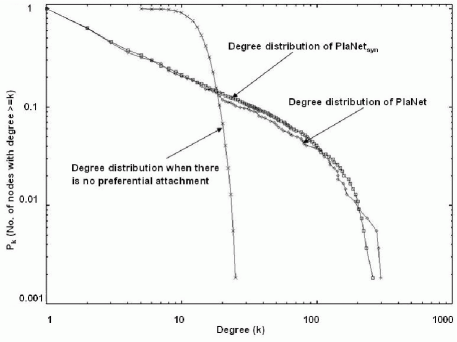
Figure 8: Degree distribution of the nodes in V_C for PlaNet_syn, PlaNet, as well as when the model incorporates no preferential attachment; for PlaNet_syn, $\epsilon$ = 0.5, $\alpha$ = 1.44, and the results are averaged over 100 simulation runs.

The mean error between the degree distribution plots of PlaNet and PlaNet_syn is $\sim$ 0.01. The match degrades as we reduce the value of $\alpha$ to 1 (linear preferential attachment) where the mean error is 0.03. The match further degrades as we continue to reduce the value of $\alpha$ and is worst for $\alpha$ = 0 (i.e., there is no preferential attachment incorporated in the model and all connections are equiprobable) where the mean error is as high as 0.35.

After having studied the properties of PlaNet_syn as discussed above, we now construct PhoNet_syn from it in the approach outlined in section 2. Next, the degree distribution as well as the clustering coefficient of PhoNet_syn is compared with that of PhoNet. Figure 9 illustrates the degree $k$ versus $P_{k}$ plot for PhoNet_syn (along with that of PhoNet). It is clear from the figure that the degree distribution curves for PhoNet and PhoNet_syn are qualitatively similar, although there is a significant amount of quantitative difference between the two (mean error $\sim$ 0.45). Moreover, the average clustering coefficient $c^{{}^{\prime}}_{av}$ of PhoNet_syn (0.55) differs largely from that of PhoNet (0.89).

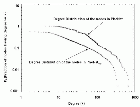
Figure 9: Degree distribution of the nodes of PhoNet_syn and PhoNet in log-log scale.

Due to this large deviation from the real data, our synthesis model needs to be refined so that it not only mimics the degree distribution of PlaNet but also reproduces the degree distribution as well as the average clustering coefficient of PhoNet. The primary reason for this deviation in the results is that the high degree of clustering, observed in PhoNet, is not taken into account by our synthesis model. Such a high clustering is a consequence of the fact that apart from preferential attachment there is some other force governing the structure of the consonant inventories. Mukherjee et al. (?, ?) reports that this force tends to bind a set of consonants in cohesive groups which essentially leads to the emergence of a pattern of co-occurrence (resulting in high clustering) among them.

Therefore, in order to boost up the clustering coefficient we refine the model to allow the formation of triads (i.e., fully connected triplets). This technique has been used by several models in the past (?, ?), which has led to increased clustering, closer to what is found in real networks. The refinement can be achieved in our model by having a language node L_j attach to some node C${}_{i}\in$ V_C if it has already attached itself to a neighbor of C_i. Two consonant nodes C₁ and C₂ are neighbors if a language node (other than L_j) attaches itself to both C₁ and C₂ in an earlier step of the synthesis process. This phenomenon leads to the formation of a large number of triangles and/or triads in the one-mode projection, which in turn is expected to yield a higher clustering coefficient.

In this model we denote the probability of triad formation by $p_{t}$. At each time step a language node L_j (chosen from the set of language nodes sorted in ascending order of their degrees) makes the first connection to some consonant node C_i $\in$ V_C (L_j is not already connected to C_i) preferentially following the distribution $Pr(C_{i})$ (specified in equation 5). For the rest of the ($k_{j}$-1) connections the language node L_j attaches itself preferentially to only the neighbors of C_i (to which L_j is not already connected) with a probability $p_{t}$. Consequently, L_j connects itself preferentially to the non-neighbors of C_i (to which L_j is not already connected) with a probability (1-$p_{t}$). Accordingly, the neighbor set of $C_{i}$ gets updated.

The entire idea mentioned above is summed up in Algorithm 2. Figure 10 shows a partial step of the synthesis process illustrated in Algorithm 2.

Algorithm 2: The refined synthesis process
Input: Nodes L1 through L317 sorted in ascending
order of their cardinalities;
for $t$ = 1 to 317 {
Choose (in order) a node Lj with cardinality kj;
Connect Lj to a node Ci $\in$ VC with which it is
not yet connected, following the distribution,
$Pr(C_{i})=\frac{{d_{i}}^{\alpha}+\epsilon}{\sum_{{i^{{}^{\prime}}}\in V^{{}^{\prime}}_{C}}({d_{i^{{}^{\prime}}}}^{\alpha}+\epsilon)}$
where V${}^{{}^{\prime}}_{C}$ is the set of nodes in VC to which Lj
is not already connected;
for $c$ = 2 to $k_{j}$ {
Connect Lj with a probability $p_{t}$ to a neigh-
bor C${}^{{}^{\prime}}_{i}$ of the node Ci (to which Lj is not yet
connected) following the distribution $Pr(C^{{}^{\prime}}_{i})$;
and,
Connect Lj with probability (1-$p_{t}$) to a non-
neighbor C${}^{{}^{\prime\prime}}_{i}$ of the node Ci (to which Lj is
not yet connected) following the distribution
$Pr(C^{{}^{\prime\prime}}_{i})$ and accordingly expand the neighbor
list of Ci;
}
}

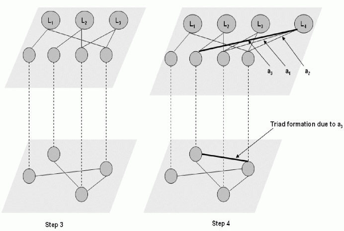
Figure 10: A partial step of the synthesis process. If the language node L₄ (which has degree 3) has the initial connection $a_{1}$ (due to preferential attachment) then according to the synthesis model the following connections would be $a_{2}$ and $a_{3}$ respectively in that order. This series of connections increases the co-occurrence by allowing formation of triads in the one-mode projection. The bold line in the figure indicates the edge that completes the triad.

3.1 Estimation of Model Parameters

The refined model discussed in Algorithm 2 involves three different parameters namely $p_{t}$, $\alpha$, and $\epsilon$. Thus at this point it becomes necessary to figure out how these model parameters interact and thereby influence the results. For this purpose we perform simulations of the model for different values of $p_{t}$ (in the range [0.7,0.95]), $\alpha$ (in the range [1.1,1.5]), and $\epsilon$ (in the range [0.2,0.4]) and study the pairwise relationships between errors that show up in (1) the degree distribution of PlaNet_syn, (2) the degree distribution of PhoNet_syn, and (3) the average clustering coefficient of PhoNet_syn.

Figure 11 shows that the mean error between the degree distribution of the pair PlaNet/PlaNet_syn is negatively correlated to that of PhoNet/PhoNet_syn. Each point on the plot indicates a certain combination of the values of $p_{t}$, $\alpha$, and $\epsilon$. Some of the non-dominating (?, ?) points are indicated by black circles in the figure.

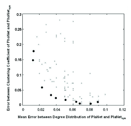
Figure 11: The correlation of the mean error between the degree distribution of PlaNet/PlaNet_syn with that of PhoNet/PhoNet_syn. Each point on the plot indicates a certain combination of the values of $p_{t}$, $\alpha$, and $\epsilon$. Some of the non-dominating points are indicated by the black circles.

Moreover, the mean error between the degree distribution of PlaNet/PlaNet_syn is also negatively correlated to the error between the average clustering coefficient of PhoNet/PhoNet_syn. Figure 12 illustrates this negative correlation. In this case again each point on the plot indicates a certain combination of the values of $p_{t}$, $\alpha$, and $\epsilon$. Some of the non-dominating points are marked by black circles in the figure.

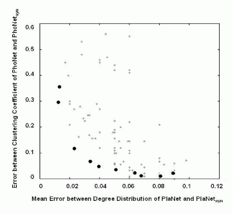
Figure 12: The correlation of the mean error between the degree distribution of PlaNet/PlaNet_syn with that of PhoNet/PhoNet_syn. Each point on the plot indicates a certain combination of the values of $p_{t}$, $\alpha$, and $\epsilon$. A few of the non-dominating points are marked by the black circles.

Further, the mean error between the degree distribution of PhoNet/PhoNet_syn and the error between the average clustering coefficient of PhoNet/PhoNet_syn do not show a direct dependence on one another (so that their effects could be assumed to be proportional), even though they are not strictly negatively correlated.

3.1.1 Combining the Objective Functions

In a multi-objective scenario as discussed above, the most common technique, reported in literature (?, ?), to arrive at a solution is to look for trade-offs rather than a single point that optimizes all the objective functions. One of the popular ways for such a trade-off is to combine (usually linearly) the objective functions together to result in a single objective function. In similar lines, we define the error $E$ which is the average of the mean error (say $M_{E}$) between degree distribution of PlaNet and PlaNet_syn, the mean error (say $M^{{}^{\prime}}_{E}$) between the degree distribution of PhoNet and PhoNet_syn, and the error (say $C_{E}$) in the average clustering coefficient of PhoNet and PhoNet_syn. In other words,

$$E=\frac{1}{3}\left(M_{E}+M^{{}^{\prime}}_{E}+C_{E}\right)$$ (6)

It is to be noted that there can be multiple other ways of combining the above three errors and equation 6 is just one of them. Having defined the error $E$, we perform a detailed study of the parameter space in order to compute the minimum value of $E$.

3.1.2 Experiment to Compute the Minimum Error

We simulate the above synthesis model with different values of $\alpha$ ranging from 1.1 to 1.5 (in steps of 0.1) and $p_{t}$ ranging from 0.70 to 0.95 (in steps of 0.05) and compute the error $E$ in each case. Figure 13 shows the three dimensional plot with $p_{t}$ in the x-axis, $\alpha$ in the y-axis and $E$ in the z-axis for three different values of $\epsilon$ which are 0.2, 0.3 and 0.4 respectively. We do not report the results for $\alpha~{}>~{}1.5$ since at larger values of $\alpha$ the error $E$ continuously keeps on rising mainly due to gelation (a condition where a single dominant “gel” node is connected to all other nodes) (?, ?). Moreover, a reasonable amount of triad formation can only take place at higher values of $p_{t}$ and hence we do not report the results for $p_{t}~{}<~{}0.70$. Further, we do not choose larger values of $\epsilon$ since it is a smoothing parameter. The figure clearly shows that in our inspection range the minimum error ($E$ = 4.1$\%$) is achieved when the values of $p_{t}$, $\alpha$ and $\epsilon$ are 0.8, 1.3 and 0.3 respectively. We have also empirically observed that these parameters are stable in the sense that a slight perturbation in them brings only a negligible change in the results.

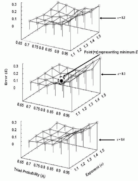
Figure 13: The error $E$ for different values of the parameters $p_{t}$, $\alpha$ and $\epsilon$. The letter $z$ indicates the point where $E$ is minimum.

3.2 Simulation Results

We plug in the best values (corresponding to minimum $E$) of the parameters $p_{t}$, $\alpha$ and $\epsilon$ as obtained in the earlier section in Algorithm 2 to synthesize PlaNet_syn and subsequently PhoNet_syn. The results of this simulation are provided below.

Figure 14 shows the degree distribution of the consonant nodes of PlaNet_syn in comparison with that of PlaNet. The mean error between the two distributions is 0.04 approximately and is therefore a deterioration from the earlier result. This is mainly due to the trade-off involved in the definition of $E$. Nevertheless, the average clustering coefficient of PhoNet_syn in this case is 0.85 as compared to 0.89 of PhoNet. Moreover, in this process the mean error between the degree distribution of PhoNet_syn and PhoNet (as illustrated in Figure 15) has got reduced dramatically from 0.45 to 0.03.

The above results equivocally indicate that for a good choice of the parameters (described earlier) the refined version of the synthesis model not only reproduces the degree distribution of PlaNet but also the degree distribution as well as the average clustering coefficient of PhoNet to a very close approximation.

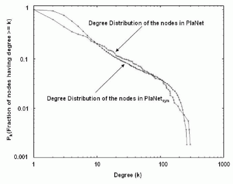
Figure 14: Degree distribution of PlaNet_syn along with that of PlaNet in log-log scale. The values of the parameters $p_{t}$, $\alpha$ and $\epsilon$ are 0.8, 1.3 and 0.3 respectively.

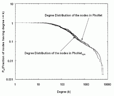
Figure 15: Degree distribution of PhoNet_syn along with that of PhoNet in log-log scale. The values of the parameters $p_{t}$, $\alpha$ and $\epsilon$ are 0.8, 1.3 and 0.3 respectively.

4 Conclusions, Discussion and Future Work

In this article we have analyzed and synthesized the consonant inventories of the world’s languages through a complex network approach. We dedicated the preceding sections for the following,

• Propose complex network representations of the consonant inventories, namely PlaNet and PhoNet,

• Provide a systematic study of some of the important structural properties of PlaNet and PhoNet,

• Develop a synthesis model for PlaNet based on preferential attachment where the consonant inventory size distribution is known a priori,

• Refine the synthesis model so that it not only mimics the degree distribution of the consonant nodes of PlaNet as well as PhoNet but also reproduces the clustering coefficient of PhoNet to a very close approximation.

Until now we have been mainly dealing with the computational aspects of the distribution of consonants over the languages rather than exploring the real world dynamics that gives rise to such a distribution. Language is a constantly changing phenomena and its present structure is determined by its past evolutionary history. The sociolinguist Jennifer Coates remarks that this linguistic change occurs in the context of linguistic heterogeneity. She explains that “. . . linguistic change can be said to have taken place when a new linguistic form, used by some sub-group within a speech community, is adopted by other members of that community and accepted as the norm.” (?, ?). In this process of language change (at the microscopic level), consonants belonging to languages that are more prevalent among the speakers in one generation have higher chances of being transmitted to the speakers of languages of the subsequent generations (?, ?, ?). In the mesoscopic level this heterogeneity in the choice of the consonants manifests itself as preferential attachment. Further, if two consonants largely co-occur in the languages of one generation, it is highly likely that they will be transmitted together in the languages of the following generations (?, ?). The aforementioned phenomenon is what is reflected through the formation of triads discussed in the earlier section. It is interesting to note that whereas triad formation among consonants takes place in a top-down fashion as a consequence of language change over linguistic generations, the same happens in a social network in a bottom-up fashion where actors come to know one another through other actors and thereby slowly shape the structure of the whole network. Moreover, unlike in a social network where a pair of actors can regulate (break or acquire) their relationship bonds, if the co-occurrence bond between two consonants breaks due to pressures of language change it can be never acquired again. Such a bond breaks only if one or both of the consonants are completely lost in the process of language change and is never formed in future since the consonants that are lost do not reappear again. In this context, Darwin in his book, The descent of man (?, ?), writes “A language, like a species, when once extinct never reappears.”

Although the directions of growth in a social network is different from the networks discussed in this article, both of them target to achieve the same configuration. It is mainly due to this reason that the principle of preferential attachment along with that of triad formation is able to capture the self-organizing behavior of the consonant inventories.

In this article we have mainly dealt with the unlabeled synthesis (since the consonant nodes are unlabeled in our synthesis model) of the occurrence and co-occurrence networks of consonants. However, the work can be further extended in the directions of a labeled synthesis of the consonant networks (and hence consonant inventories). We look forward to accomplish the same as a part of our future work.

References

- Abrams and StrogtzAbrams and Strogtz Abrams, D. M. and Strogatz, S. H. (2003). Modelling the dynamics of language death. Nature 424, 900.
- Abraham et alAbrams et al Abraham, A., Jain, L. C. and Goldberg, R. (2005). Evolutionary multiobjective optimization: Theoretical advances and applications, Springer–Verlag.
- Albert and BarabásiAlbert and Barabási Albert, R. and Barabási, A.-L. (2002). Statistical mechanics of complex networks. Reviews of Modern Physics 74, 47–97.
- Arhem et alArhem et al Arhem, P., Braun, H. A., Huber, M. T. and Liljenstrom, H. (2004). Micro-Meso-Macro: Addressing complex systems couplings, World Scientific.
- Barabási and AlbertBarabási and Albert Barabási, A.-L. and Albert, R. (1999). Emergence of scaling in random networks. Science 286, 509- 512.
- Barrat et alBarrat et al Barrat, A., Barthélemy, M., Pastor-Satorras, R. and Vespignani, A. (2004). The architecture of complex weighted networks. PNAS 101, 3747–3752.
- Baxter et alBaxter et al Baxter, G. J., Blythe, R. A., Croft, W. and McKane, A. J. (2006). Utterance selection model of language change. Physical Review E 73, 046118.
- BhattBhatt Bhatt, D. N. S. (2001). Sound Change, Motilal Banarsidass, New Delhi.
- BlevinsBlevins Blevins, J. (2004). Evolutionary phonology: The emergence of sound patterns, Cambridge University Press.
- de Boerde Boer de Boer, B. (2000). Self-organisation in vowel systems. Journal of Phonetics 28(4), 441–465.
- BoersmaBoersma Boersma, P. (1998). Functional phonology, Doctoral thesis, University of Amsterdam, The Hague: Holland Academic Graphics.
- BulmerBulmer Bulmer, M. G. (1979). Principles of statistics, Mathematics.
- Cancho and SoléCancho and Solé Ferrer i Cancho, R. and Solé, R. V. (2001). The small-world of human language. Santa Fe working paper 01-03-016.
- CoatesCoates Coates, J. (1993). Women, men and language, London: Longman.
- ClementsClements Clements, N. (2004). Features and sound inventories. Symposium on Phonological Theory: Representations and Architecture, CUNY.
- DarwinDarwin Darwin, C. R. (1871). The descent of man, and selection in relation to sex, London: John Murray.
- FlemmingFlemming Flemming, E. (2002). Auditory representations in phonology, New York and London: Routledge.
- Hinskens and WeijerHinskens and Weiger Hinskens, F. and Weijer, J. (2003). Patterns of segmental modification in consonant inventories: A cross-linguistic study. Linguistics 41, 6.
- Jeong et alJeong et al Jeong, H., Tombor, B., Albert, R., Oltvai, Z. N. and Barabási, A.-L. (2000). The large-scale organization of metabolic networks. Nature 406, 651 -654.
- Ladefoged and MaddiesonLadefoged and Maddieson Ladefoged, P. and Maddieson, I. (1996). Sounds of the world s languages, Oxford: Blackwell.
- LightfootLightfoot Lightfoot, D. (1999). The development of language: Acquisition, change and evolution, Oxford: Blackwell.
- Lindblom and MaddiesonLindblom and Maddieson Lindblom, B. and Maddieson, I. (1988). Phonetic universals in consonant systems. Language, Speech, and Mind, 62–78, Routledge, London.
- MaddiesonMaddieson Maddieson, I. (1984). Patterns of sounds, Cambridge University Press, Cambridge.
- MaddiesonMaddieson Maddieson, I. 1999. In search of universals. Proceedings of the XIVth International Congress of Phonetic Sciences, 2521 -2528.
- Mukherjee et alMukherjee et al Mukherjee, A., Choudhury, M., Basu, A. and Ganguly, N. (2007). Modeling the co-occurrence principles of the consonant inventories: A complex network approach. Int. Jour. of Mod. Phys. C, 18(2), 281–295.
- NewmanNewman Newman, M. E. J. (2001). Scientific collaboration networks. Phys. Rev. E 64.
- NewmanNewman Newman, M. E. J. (2003). The structure and function of complex networks. SIAM Review 45, 167–256.
- OudeyerOudeyer Oudeyer, P. (2006). Self-organization in the evolution of speech, Oxford University Press.
- Peltomäki and AlavaPeltomäki and Alava Peltomäki, M. and Alava, M. (2006). Correlations in bipartite collaboration networks. Journal of Statistical Mechanics: Theory and Experiment, Issue 1, 01010.
- Pericliev and Valdés-PérezPericliev and Valdés-Pérez Pericliev, V. and Valdés-Pérez, R. E. (2002). Differentiating 451 languages in terms of their segment inventories. Studia Linguistica 56(1), 1–27.
- Ramasco et alRamasco et al Ramasco, J. J., Dorogovtsev, S. N. and Pastor-Satorras, R. (2004). Self-organization of collaboration networks. Physical Review E 70, 036106.
- SimonSimon Simon, H. A. (1955). On a class of skew distribution functions. Biometrika 42, 425 -440.
- StampeStampe Stampe, D. (1973). A dissertation on natural phonology, PhD dissertation, University of Chicago.
- TrubetzkoyTrubetzkoy Trubetzkoy, N. (1969). Principles of phonology. (English translation of Grundzüge der Phonologie, 1939), Berkeley: University of California Press.
- VitevitchVitevitch Vitevitch, M. S. (2005). Phonological neighbors in a small world: What can graph theory tell us about word learning? Spring 2005 Talk Series on Networks and Complex Systems, Indiana University, Bloomington.
- Watts and StrogatzWatts and Strogatz Watts, D. J. and Strogatz, S. H. (1998). Collective dynamics of small-world networks. Nature 393, 440 -442.
- Yook et alYook et al Yook, S., Jeong, H. and Barabási, A.-L. (2001). unpublished.