Balanced vehicular traffic at a bottleneck

Abstract

The balanced vehicular traffic model is a macroscopic model for vehicular traffic flow. We use this model to study the traffic dynamics at highway bottlenecks either caused by the restriction of the number of lanes or by on-ramps or off-ramps. The coupling conditions for the Riemann problem of the system are applied in order to treat the interface between different road sections consistently. Our numerical simulations show the appearance of synchronized flow at highway bottlenecks.

1 Introduction

The balanced vehicular traffic model (BVT model), which was first introduced in [10], generalizes the macroscopic traffic model of Aw, Rascle [1, 13] and Greenberg [3] by introducing an effective relaxation coefficient into the momentum equation of traffic flow. This effective relaxation coefficient can become negative, resulting in multivalued fundamental diagrams in the congested regime. Such negative effective relaxation coefficients follow from finite reaction and relaxation times of drivers (see [10]). For related ideas, see Greenberg-Klar-Rascle [5], Greenberg [4].

In a previous work [11] we studied the behavior of the BVT model at a bottleneck. There, we manipulated the partial differential equations describing traffic flow at the bottleneck by artificially resetting the average velocity in order to model a speed restriction. The results obtained in that study showed the basic behavior of the BVT model and its potential to explain the observed patterns of traffic flow [9]. Although the procedure of resetting quantities, i.e. the average velocity in that case, was locally restricted, it leaves the question whether the model can adequately describe synchronized flow at a bottleneck. In order to show this, the current paper systematically studies the traffic dynamics at highway bottlenecks in the BVT model by numerical means. To do this in agreement with the underlying partial differential equations we use the coupling conditions for the Riemann problems at the interface between different highway sections. We focus the discussion on two setups: In the first setup we study a bottleneck caused by the narrowing of a highway from three lanes to two lanes. In the second setup we study a two-lane highway with an on-ramp and an off-ramp.

The outline of the paper is as follows. In Section 2 we summarize the theory of the coupling conditions for the Riemann problem at intersections. Whereas Section 3 presents numerical results for a highway bottleneck caused by the restriction of the number of lanes from three lanes to two lanes, Section 4 presents the numerical results for a two-lane highway with an on-ramp and an off-ramp. In Section 5 we introduce the possible generalization to an arbitrary junction. We finally summarize our results in Section 6.

2 Coupling conditions

Before we have a closer look at the coupling conditions, let us repeat the principal equations of the BVT model. The evolution equations for the density $\rho$ of vehicles and the average velocity $v$ are described by the following hyperbolic system of balance laws

$$\frac{\partial\rho}{\partial t}+\frac{\partial(\rho v)}{\partial x} = 0,$$ (1)

$$\frac{\partial(\rho(v-u(\rho))}{\partial t}+\frac{\partial(\rho v(v-u(\rho)))}{\partial x} = b(\rho,v){\rho(u(\rho)-v)}.$$ (2)

Here, $u(\rho)$ denotes the equilibrium velocity, therefore the expression $v-u(\rho)=w$ describes a distance to equilibrium. The quantity $b(\rho,v)$ is the effective relaxation coefficient. For the case where $b(\rho,v)$ becomes negative, there are additional equilibrium velocities, i.e. high-flow branch and the jam line. Whereas the high-flow branch is metastable for intermediate densities and unstable for high densities, the jam line is unstable for intermediate densities and metastable for high densities. For a detailed discussion see [11]. Note that the pseudo-momentum $\rho(v-u(\rho))$ is not conserved due to the non-vanishing term on the right-hand side of Eqn. (2). This source term plays an essential role for the traffic dynamics on road sections, but it is neglected for the situation where one is interested in the Riemann problems at intersections, since it is never a delta-function.

2.1 Background

Piccoli and Garavello [2] appear to have been the first to propose an intersection modeling by using the Aw-Rascle “second order” model of traffic flow [1]. In their approach, only the mass flux is conserved but not the pseudo-momentum. In [8], Herty and Rascle proposed another approach in which mass flux and pseudo-momentum are both conserved. But they maximized the mass fluxes at the intersection with some arbitrary given homogenization coefficients. In [7], the latter approach has been generalized by maximizing the total mass flux at the junction without fixing any condition. In fact, the homogenization coefficients are not arbitrary but obtained directly from the mass flux maximization. Another approach also based on the mass flux maximization is given in [6]. Our approach in the current paper is similar to the latter one, in particular we maximize the total flux at the junction, at the same time conserving the pseudo-momentum of the original “Aw-Rascle” system. Here, we are particularly concerned with the BVT model [10]. We note that our treatment of the homogenization problem which naturally arises in a merge junction is different from the one in [8],[7], see Remark 1.

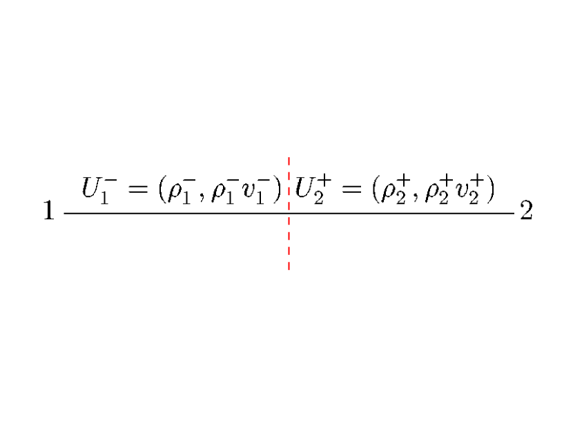
a)

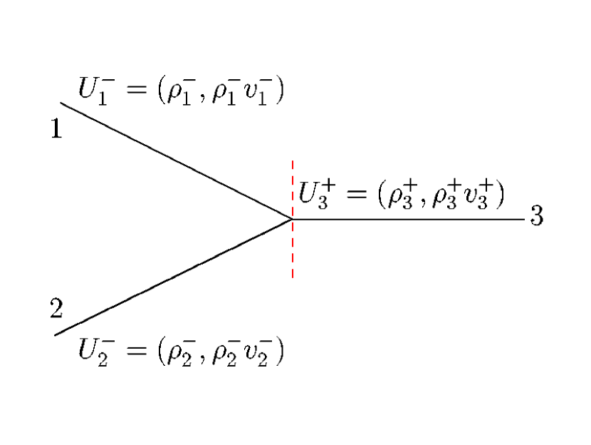
b)

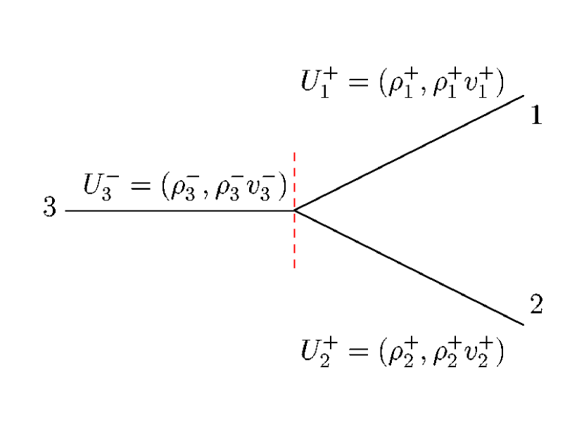
c)

Figure 1: Definition of the quantities at junctions, which are necessary to construct the boundary fluxes. The junction in a) consists of one incoming and one outgoing road. The panels b) and c) display a merge junction and a diverge junction, respectively. The direction of the flow is from left to right.

2.2 Junction consisting of one incoming and one outgoing road

In the following we restrict the discussion to the Riemann problem at the interface between two road sections. The road section 1 is located upstream and the road section 2 downstream of the interface, where the flux functions have to be determined. Let $U_{1}^{-}=(\rho_{1}^{-},\rho_{1}^{-}v_{1}^{-})$ be the state vector at the interface upstream in the road section 1 and let $U_{2}^{+}=(\rho_{2}^{+},\rho_{2}^{+}v_{2}^{+})$ be the state vector at the interface downstream in the road section 2 (see panel a) of Fig. 1). For each road section $j$ we introduce the function $w_{j}$ of the state variable $U=(\rho,\rho v)$

$$w_{j}(U)=v-u_{j}(\rho).$$ (3)

According to Herty and Rascle [8] the fluxes at the interface between the two road sections (see Eqs. (1)-(2))

$$\hat{f}=q\left(\begin{array}[]{c}1\\ w_{1}(U_{1}^{-})\end{array}\right)$$ (4)

can be calculated from the expression

$$q=\min(d_{1}(\rho_{1}^{-}),s_{2}(\rho_{2}^{\dagger})),$$ (5)

where the demand and supply functions $d_{1}(\rho)$ and $s_{2}(\rho)$ and the density $\rho_{2}^{\dagger}$ are defined below.

The density $\rho_{2}^{\dagger}$ is defined as the intersection point of the two curves $v=v_{2}^{+}$, $w_{2}(U)=w_{1}(U_{1}^{-})$ and can be obtained by solving the implicit equation

$$u_{2}(\rho_{2}^{\dagger})-v_{2}^{+}+w_{1}(U_{1}^{-})=0.$$ (6)

Let us define the function

$$\eta_{d1}(\rho)=\rho u_{1}(\rho)+\rho w_{1}(U_{1}^{-}).$$ (7)

For a monotonously decreasing, differentiable function $u_{1}(\rho)$ the function $\eta_{d1}(\rho)$ has a single maximum at location $\tilde{\rho}_{1}$, which can be obtained by solving the implicit equation

$$\eta_{d1}^{\prime}(\tilde{\rho}_{1})=\tilde{\rho}_{1}u^{\prime}_{1}(\tilde{\rho}_{1})+u_{1}(\tilde{\rho}_{1})+w_{1}(U_{1}^{-})=0.$$ (8)

It is now possible to define the demand function

$$d_{1}(\rho)=\begin{cases}\eta_{d1}(\rho),&\text{if $\rho\leq\tilde{\rho}_{1}$,}\\ \eta_{d1}(\tilde{\rho}_{1}),&\text{if $\rho>\tilde{\rho}_{1}$.}\end{cases}$$ (9)

Let us define the function

$$\eta_{s2}(\rho)=\rho u_{2}(\rho)+\rho w_{1}(U_{1}^{-}).$$ (10)

For a monotonously decreasing, differentiable function $u_{2}(\rho)$ the function $\eta_{s2}(\rho)$ has a single maximum at location $\tilde{\rho}_{2}$, which is determined by solving the implicit equation

$$\eta_{s2}^{\prime}(\tilde{\rho}_{2})=\tilde{\rho}_{2}u^{\prime}_{2}(\tilde{\rho}_{2})+u_{2}(\tilde{\rho}_{2})+w_{1}(U_{1}^{-})=0.$$ (11)

With this function we define the supply function as

$$s_{2}(\rho)=\begin{cases}\eta_{s2}(\tilde{\rho}_{2}),&\text{if $\rho<\tilde{\rho}_{2}$,}\\ \eta_{s2}(\rho),&\text{if $\rho\geq\tilde{\rho}_{2}$.}\end{cases}$$ (12)

We numerically solve the implicit Eqs. (8) and (11) using the method of nested intervals. With the expression for the fluxes at the interface between the two road sections (see Eqn. (4)), we obtain the necessary boundary values at the interface for the conservative update scheme described in detail in [10].

2.3 Merge junction

We are now interested in the boundary fluxes at a merge junction, see panel b) of Fig. 1. In order to define the demand functions on the incoming road sections $i=1,2$ we first define the functions $\eta_{di}(\rho)$ as follows,

$$\eta_{di}(\rho)=\rho u_{i}(\rho)+\rho w_{i}(U_{i}^{-}).$$ (13)

Let us denote the maxima of the corresponding curves as ${\tilde{\rho}}_{i}$. We can then define the demand function of the road section $i$ as

$$d_{i}(\rho)=\begin{cases}\eta_{di}(\rho),&\text{if $\rho\leq\tilde{\rho}_{i}$,}\\ \eta_{di}(\tilde{\rho}_{i}),&\text{if $\rho>\tilde{\rho}_{i}$.}\end{cases}$$ (14)

In order to define the supply function in the road section 3, we first introduce quantities $\beta_{i}$ describing the fraction of cars entering from the road section $i$ into the road section 3. When we assume that the incoming fluxes passing through the junction are proportional to the incoming demands, we have

$$\beta_{i}=\frac{d_{i}(\rho_{i}^{-})}{\sum_{j=1}^{2}d_{j}(\rho_{j}^{-})}.$$ (15)

With this definition, we follow [6] and do not consider these fractions as part of the optimization problem as in [7]. We define the homogenized value $w_{3}^{*}$ for the quantity $w$ defined in Eqn. (3), i.e.

$$w_{3}^{*}=\sum_{j=1}^{2}\beta_{j}w_{j}(U_{j}^{-}),$$ (16)

and with the latter the function

$$\eta_{s3}(\rho)=\rho u_{3}(\rho)+\rho w_{3}^{*}$$ (17)

which reaches its maximum value at $\tilde{\rho}_{3}$.

Remark 1

Here, we assume that the velocity on road 3, near the junction, is given by $v=u_{3}(\rho)+w_{3}^{*}$. This is in contrast with [8] and [7], where the mixture of cars from both incoming roads 1 and 2 is assumed to produce an homogenized flow, with a nonlinear relation between $\rho$ and $v$ which expresses that the cars from roads 1 and 2 microscopically share the available space. The resulting mixture rule is more appropriately described in Lagrangian (mass) coordinates, but is definitely not in the above form.

In other words, the assumptions in [8] and [7] are incompatible with the (simpler) formula (17), which we assume here. Naturally, in practice the difference is not necessarily significant. We will come back to this point elsewhere.

We are now able to define the supply function

$$s_{3}(\rho)=\begin{cases}\eta_{s3}(\tilde{\rho}_{3}),&\text{if $\rho<\tilde{\rho}_{3}$,}\\ \eta_{s3}(\rho),&\text{if $\rho\geq\tilde{\rho}_{3}$.}\end{cases}$$ (18)

This function will be evaluated below at the intersection point of the two curves $v=v_{3}^{+}$ and $w_{3}(U)=w_{3}^{*}$, which corresponds to a density $\rho_{3}^{\dagger}$ fulfilling the implicit equation

$$u_{3}(\rho_{3}^{\dagger})-v_{3}^{+}+w_{3}^{*}=0.$$ (19)

Finally, we define the downstream boundary fluxes in the road section $i$ as

$$\hat{f}_{i}^{-}=q\beta_{i}\left(\begin{array}[]{c}1\\ w_{i}(U_{i}^{-})\end{array}\right)$$ (20)

and the upstream boundary fluxes in the road section 3 as

$$\hat{f}_{3}^{+}=q\left(\begin{array}[]{c}1\\ w_{3}^{*}\end{array}\right),$$ (21)

where

$$q=\min\Big{(}\sum_{j=1}^{2}d_{j}(\rho_{j}^{-}),s_{3}(\rho_{3}^{\dagger})\Big{)}.$$ (22)

Note that the above boundary fluxes are conserved through the intersection, and are bounded from above by the demands and supplies.

2.4 Diverge junction

In this section we study the boundary fluxes at a diverge junction, see panel c) of Fig. 1. Again we set

$$\eta_{d3}(\rho)=\rho u_{3}(\rho)+\rho w_{3}(U_{3}^{-})$$ (23)

and denote the maximum of that function as $\tilde{\rho}_{3}$. The demand function in the road section 3 is defined as

$$d_{3}(\rho)=\begin{cases}\eta_{d3}(\rho),&\text{if $\rho\leq\tilde{\rho}_{3}$,}\\ \eta_{d3}(\tilde{\rho}_{3}),&\text{if $\rho>\tilde{\rho}_{3}$.}\end{cases}$$ (24)

For the definition of the supply function we first have to prescribe the fractions of cars intending to enter from road section 3 into road section 1 and road section 2, which we describe with the quantities $\alpha_{31}$ and $\alpha_{32}$. We stress that these quantities - in contrast to [6] - need not agree with the actual percentages of the flow from road section 3 entering into road section 1 and road section 2, see Eqs. (31)-(34) below. Under the assumption that all cars remain in the network, i.e. $\alpha_{31}+\alpha_{32}=1$, we can set

$$\alpha_{31} = \alpha,$$ (25)

$$\alpha_{32} = (1-\alpha),$$ (26)

with $\alpha\in[0,1]$. For the outgoing roads sections $k=1,2$ we define

$$\eta_{sk}=\rho u_{k}(\rho)+\rho w_{3}(U_{3}^{-})$$ (27)

and denote the maxima of these functions $\tilde{\rho}_{k}$. The supply function on the outgoing road section $k$ then reads

$$s_{k}(\rho)=\begin{cases}\eta_{sk}(\tilde{\rho}_{k}),&\text{if $\rho<\tilde{\rho}_{k}$,}\\ \eta_{sk}(\rho),&\text{if $\rho\geq\tilde{\rho}_{k}$.}\end{cases}$$ (28)

We also have to determine the densities $\rho_{k}^{\dagger}$, at which these supply functions are evaluated. These densities are calculated from the intersection of the curves $v=v_{k}^{+}$ and $w_{k}(U)=w_{3}(U_{3}^{-})$, which reduces to the implicit equations

$$u_{k}(\rho_{k}^{\dagger})-v_{k}^{+}+w_{3}(U_{3}^{-})=0.$$ (29)

Finally, we define downstream boundary fluxes of road section 3 as

$$\hat{f}_{3}^{-}=q\left(\begin{array}[]{c}1\\ w_{3}(U_{3}^{-})\end{array}\right)$$ (30)

and the upstream boundary fluxes in road section 1 as

$$\hat{f}_{1}^{+}=q_{1}\left(\begin{array}[]{c}1\\ w_{3}(U_{3}^{-})\end{array}\right),$$ (31)

and in the road section 2 as

$$\hat{f}_{2}^{+}=q_{2}\left(\begin{array}[]{c}1\\ w_{3}(U_{3}^{-})\end{array}\right),$$ (32)

where

$$q_{1}=\min{\Big{(}\alpha d_{3}(\rho_{3}^{-}),s_{1}(\rho_{1}^{\dagger})\Big{)}},$$ (33)

$$q_{2}=\min{\Big{(}(1-\alpha)d_{3}(\rho_{3}^{-}),s_{2}(\rho_{2}^{\dagger})\Big{)}},$$ (34)

and

$$q=q_{1}+q_{2}.$$ (35)

Note again that the above boundary fluxes are conserved through the interface, and are bounded from above by the demands and supplies.

3 Lane reduction on a highway

We study the traffic dynamics for the setup depicted in Fig. 2. The highway under study consists of two 7 km long road sections. The road section 1 consists of three lanes whereas the road section 2 consists of two lanes. Note that in the mathematical description the transition from two to three lane is immediate, the length of the merging segments is neglected.

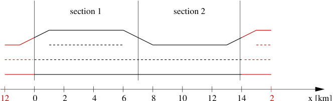
Figure 2: Sketch of the highway under study. The highway consists of two road sections of 7 km length. The road section 1 consists of three lanes whereas the road section 2 consists of two lanes. We use periodic boundary conditions, i.e. the road section 1 is also located downstream of the road section 2.

As in [11] we use the equilibrium velocity function of Newell

$$u(\rho)=u_{m}\Big{(}1-\exp\Big{(}-\frac{\lambda}{u_{m}}\Big{(}\frac{1}{\rho}-\frac{1}{\rho_{m}}\Big{)}\Big{)}\Big{)}$$ (36)

with parameter values $u_{m}=160\ {\rm km/h}$, $\lambda=3600\ {\rm[1/h/lane]}$, $\rho_{m}=160\ {\rm[1/km/lane]}$ and an effective relaxation coefficient

$$b(\rho,v)=\left\{\begin{array}[]{ll}\frac{a_{c}}{u-v},&\mbox{if~{}}\tilde{\beta}(\rho,v)(u(\rho)-v)-a_{c}\geq 0,\\ \frac{d_{c}}{u-v},&\mbox{if~{}}\tilde{\beta}(\rho,v)(u(\rho)-v)-d_{c}\leq 0,\\ \tilde{\beta}(\rho,v),&\mbox{else},\end{array}\right.$$ (37)

$$\tilde{\beta}(\rho,v)=\frac{1}{\hat{T}u_{m}}\Big{(}|u(\rho)-v+a_{1}\Delta v|+a_{2}\Delta v\Big{)}$$ (38)

and

$$\Delta v(\rho)=\tanh\Big{(}a_{3}\frac{\rho}{\rho_{m}}\Big{)}\Big{(}u(\rho)+c\rho_{m}\Big{(}\frac{1}{\rho}-\frac{1}{\rho_{m}}\Big{)}\Big{)},$$ (39)

with parameters $a_{c}=2\ {\rm m/s^{2}}$, $d_{c}=-5\ {\rm m/s^{2}}$, $\hat{T}=0.1\ {\rm s}$, $a_{1}=-0.2$, $a_{2}=-0.8$, $a_{3}=7$ and $c=-14\ {\rm km/h}$. Thus the maximum density of the road section 1 is 480 vehicles/km. The road section 2 can support 320 vehicles/km at maximum. The initial data to start the numerical simulations consists of equilibrium data on the two road sections. We prescribe a constant vehicle density $\rho_{0}$ in both road sections, setting the initial velocity to $v=u(\rho_{0})$. We choose the constant $\rho_{0}$ to be independent of the number of the lanes, the corresponding scaled densities in each road section follow from dividing $\rho_{0}$ by the number of lanes of that road section. In the following we perform a parameter study of $\rho_{0}$, varying the quantity between $50$ [1/km] and $300$ [1/km] in steps of $50$ [1/km]. Figure 3 displays the simulation results for the density (left column) and velocity (right column) for simulations covering two hours. Note that, although the initial data are in equilibrium in each road section, the coupling conditions at the interface between the two road sections do not guarantee the equilibrium during the evolution.

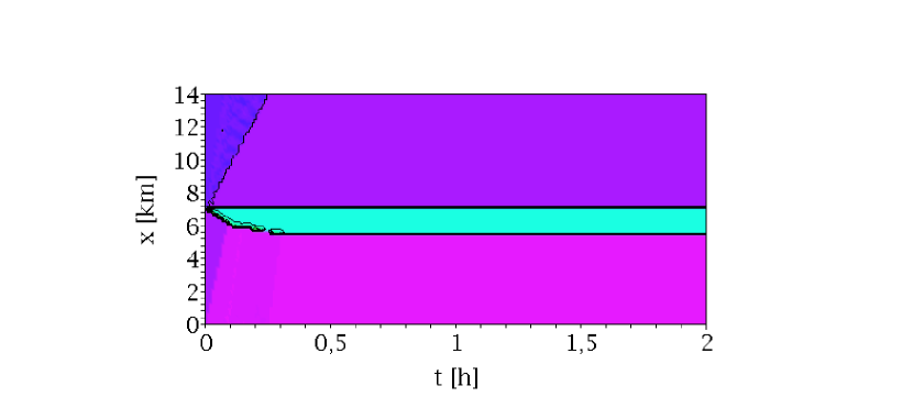
$\rho_{0}=50~{}$ [1/km]

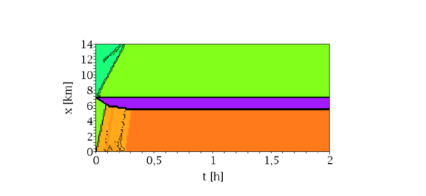
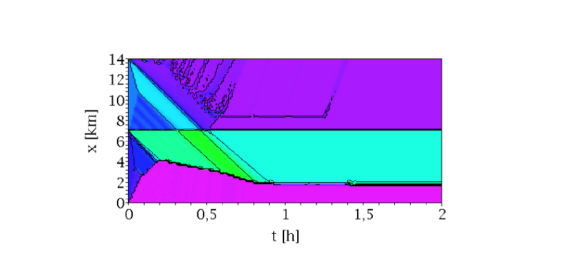
$\rho_{0}=100$ [1/km]

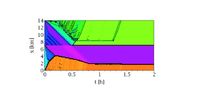
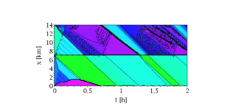
$\rho_{0}=150$ [1/km]

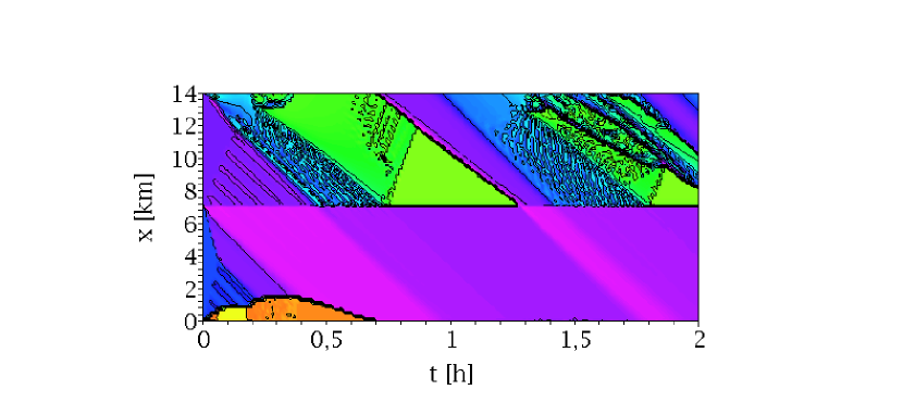
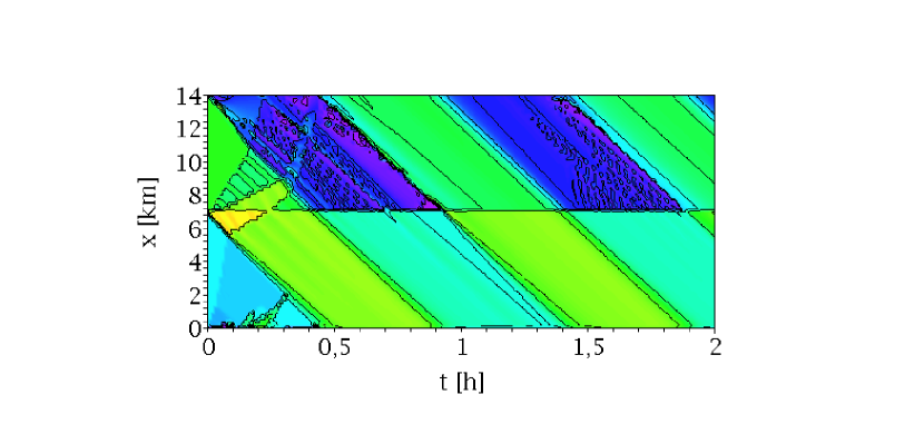
$\rho_{0}=200$ [1/km]

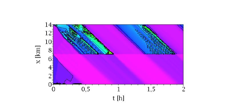
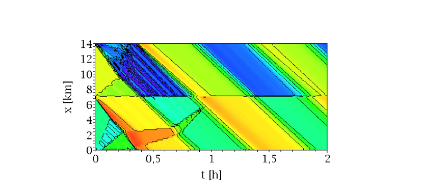
$\rho_{0}=250$ [1/km]

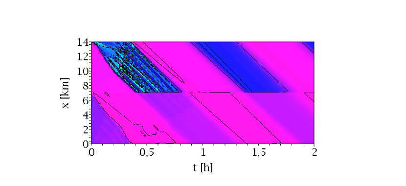
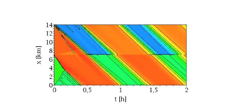
$\rho_{0}=300$ [1/km]

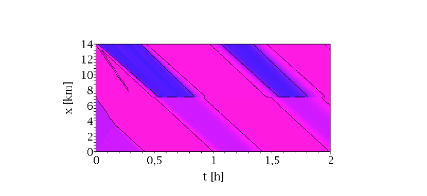
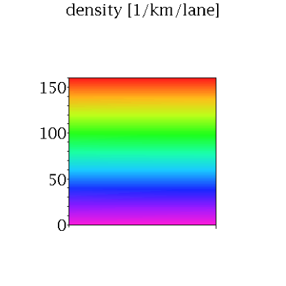
Figure 3: Traffic dynamics at the bottleneck caused by the reduction of the number of lanes on a highway. The column on the left shows the evolution of the vehicle density in units [1/km/lane], the column on the right the corresponding evolution of the velocity in units [km/h]. The different rows correspond to different simulation runs varying the initial density $\rho=\rho_{0}$ as indicated. See the text for a detailed description.

For a density $\rho_{0}=50$ [1/km], a small region of higher density and lower velocity forms between about 5.5 km and 7 km. This region corresponds to data located in the fundamental diagram on and scattered around the jam line. Clearly, this congested region is fixed at the bottleneck and therefore cannot correspond to a wide moving jam. The structure is supported by the bottleneck, i.e. the insufficient capacity of the road section 2 to carry the corresponding free flow rates in the road section 1. This region corresponds to synchronized flow. For a density $\rho_{0}=100$ [1/km], the dynamics becomes more complicated, but finally a synchronized flow region of extended width (ranging from about 2 km to 7 km) forms. Only in a small region of the road section 1 (between 0 km and 2 km) traffic is in free flow. For a density $\rho_{0}=150$ [1/km], the synchronized flow region covers the entire road section 1. Moreover, a wide moving jam travels through the two road sections, see the bright pink structure in the velocity plot. Increasing the density still further leads to even wider wide moving jams. The velocities inside these jams decrease with the increase of the initial density $\rho_{0}$. For $\rho_{0}=300$ [1/km] velocities of less than 1 [km/h] are reached inside the wide moving jam. Note that the wide moving jams are not affected by the interfaces between the two road sections of the highway. They travel upstream with an almost constant speed.

4 Bottlenecks caused by on-ramps and off-ramps

In the second setup we analyze by numerical means a two-lane highway with an on-ramp and an off-ramp. The simulation setup is displayed in Fig. 4. For our simulations we chose a length of 7 km for two-lane road sections 1 and 3 each, and a length of 10 km for the one-lane road section 2.

Figure 4: Sketch of the simulation setup. We study the dynamics on a two-lane highway with an on-ramp between the road sections 1 and 3 and an off-ramp between the road sections 3 and 1. On- and off-ramp form the boundaries of the one-lane road section 2.

For the parameterization of the equilibrium velocity curve and the effective relaxation coefficient, we use again the values given in Eqs. (36)-(39). We start the simulations with a constant density in equilibrium on all road sections of $\rho_{0}=50$ [1/km/lane] and vary the percentage of cars $\alpha$ aiming to enter the road section 1 from the road section 3, see Eqn. (25). The numerical results are summarized in Fig. 5.

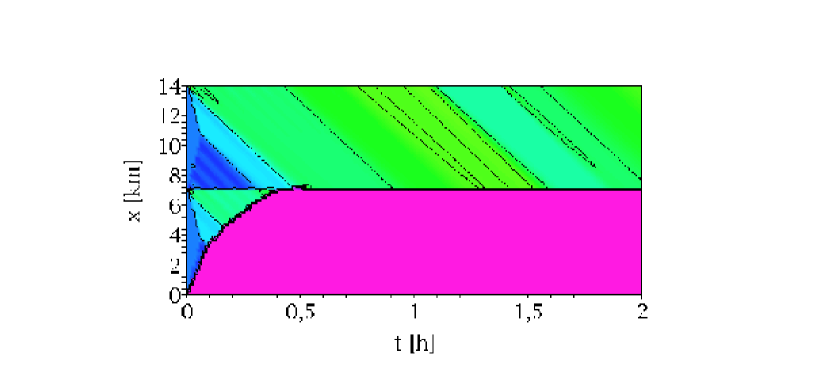
$\alpha=0.1$

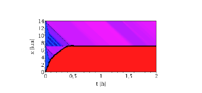
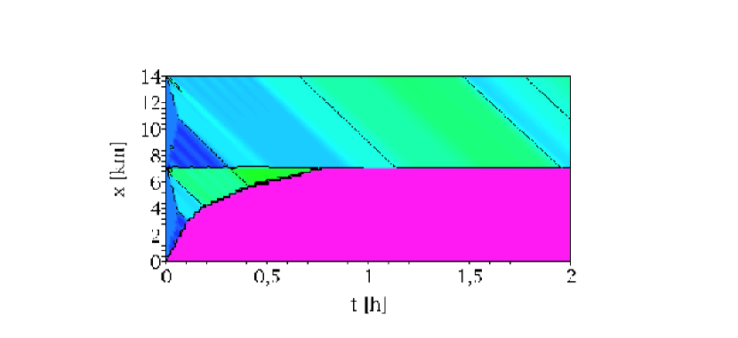
$\alpha=0.3$

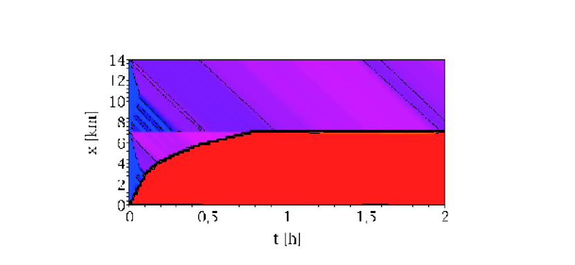
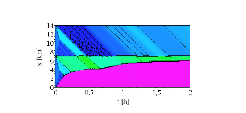
$\alpha=0.5$

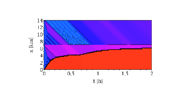
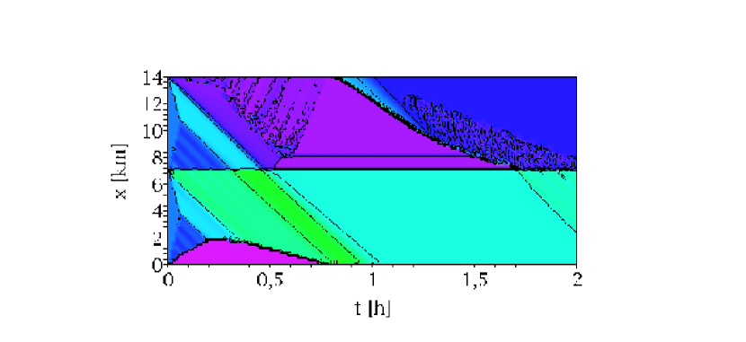
$\alpha=0.7$

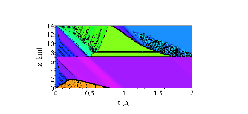
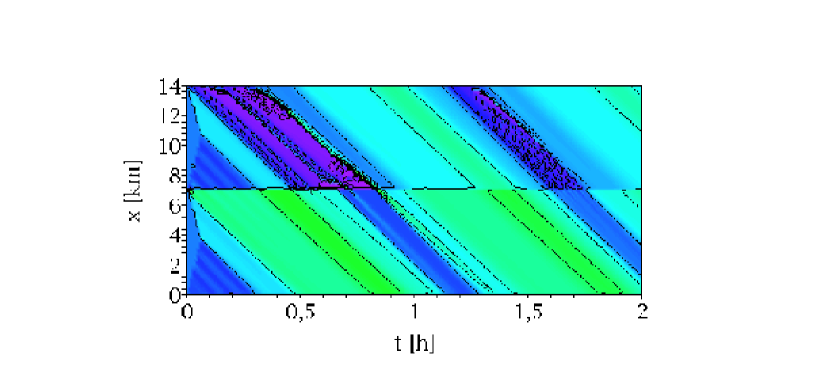
$\alpha=0.9$

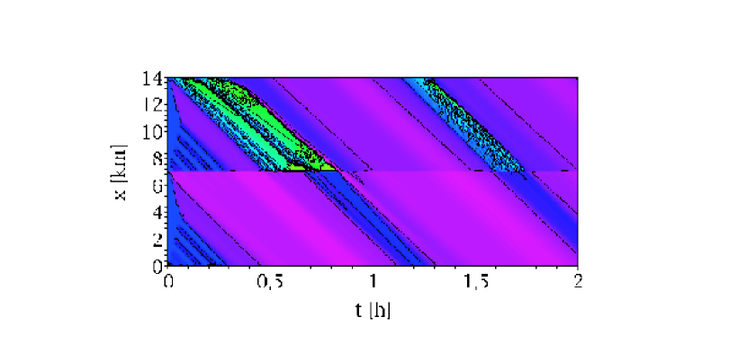
Figure 5: Traffic dynamics at highway bottlenecks caused by on-ramps and off-ramps. The plot shows the traffic dynamics on the two-lane highway, the road section 1 corresponds to the region between 0 and 7 km, the road section 3 corresponds to the region between 7 and 14 km. We vary the percentage of cars intending to enter from the road section 3 into the road section 1, i.e. the value of $\alpha$, in the range between 0.1 and 0.9 (different rows). The column on the left shows the evolution of the vehicle density in units [1/km/lane], the column on the right the corresponding evolution of the velocity in units [km/h].

For small to intermediate values of the parameter $\alpha$, the simulations develop a state, where the road section 1 is almost empty, i.e. traffic is in free flow in the road section 1. This can be easily understood by realizing that for small values of $\alpha$ most of the cars use the by-pass road section 2. In contrast, traffic is in the congested regime in the road section 3. For sufficiently high values of $\alpha$ (see the results for $\alpha=0.5$) synchronized flow develops in front of the on-ramp in the road section 1. For $\alpha=0.7$ there is only a small region of free flow remaining in road section 1 which disappears after a time of about 0.8 h. For a parameter value $\alpha=0.9$ a region of narrow moving jams forms in front of the off-ramp in the road section 3.

5 Extension to a general junction

For a given junction $n$, let us denote by $\delta^{-}_{n}$ and $\delta^{+}_{n}$, respectively the set of all incoming roads to $n$ (indexed $i$ in the sequel) and the set of all the outgoing roads to $n$ (indexed $k$ in the following). We require the equations (1)-(2) to hold on each road of $\delta_{n}^{-}\cup\delta_{n}^{+}$. The percentage of cars on the road $i$ intending to go to the road $k$ are denoted by $\alpha_{ik}$, such that $\forall i\in\delta_{n}^{-},\sum_{k}\alpha_{ik}=1$. These coefficients are assumed to be known.

Let $U_{i}^{-}=(\rho_{i}^{-},\rho_{i}^{-}v_{i}^{-}),\ \ \forall i\in\delta_{n}^{-}$ and $U_{k}^{-}=(\rho_{k}^{+},\rho_{k}^{+}v_{k}^{+}),\ \ \forall k\in\delta_{n}^{+}$, respectively the boundary values on the incoming and outgoing roads. We denote by $\beta_{ik}$, such that $\forall k\in\delta_{n}^{+},\sum_{i}\beta_{ik}=1$, the proportion of cars on the road $k$ coming from the road $i$. We set

$$\beta_{ik}=\frac{\alpha_{ik}d_{i}(\rho_{i}^{-})}{\sum_{i\in\delta_{n}^{-}}{\alpha_{ik}d_{i}(\rho_{i}^{-})}}\ \ \ \forall i\in\delta_{n}^{-},\ \forall k\in\delta_{n}^{+},$$ (40)

with the demand functions $d_{i}$ as defined in Eqs. (13)-(14). The homogenized $w$ on the outgoing roads near the junction are as follows

$$w_{k}^{*}=\sum_{i\in\delta_{n}^{-}}\beta_{ik}w_{i}(U_{i}^{-}),\ \ \ \forall k\in\delta_{n}^{+}.$$ (41)

With these quantities we define the supply functions $s_{k}$ as in Eqs. (17)-(18) for arbitrary $k\in\delta_{n}^{+}$. For all $k\in\delta_{n}^{+}$, the intermediate state of density $\rho_{k}^{\dagger}$ on the outgoing road is given by the intersection point between the curves $v_{k}(U)=v_{k}^{+}$ and $w_{k}(U)=w_{k}^{*}$.

To obtain the flux $q$ on each road one has to solve the following maximization problem

$$\max\sum_{k\in\delta_{n}^{+}}q_{k}\mbox{ subject to }$$ (42a)

$$\ 0\leq q_{i}\leq d_{i}(\rho_{i}^{-}),\forall i\in\delta_{n}^{-};$$ (42b)

$$\ 0\leq q_{k}\leq s_{k}(\rho_{k}^{\dagger}),\forall k\in\delta_{n}^{+};$$ (42c)

$$\ q_{i}=\sum_{k\in\delta_{n}^{+}}\beta_{ik}q_{k},\forall i\in\delta_{n}^{-};$$ (42d)

$$\ q_{k}\leq\sum_{i\in\delta_{n}^{-}}\alpha_{ik}d_{i}(\rho_{i}^{-}),\forall k\in\delta_{n}^{+}.$$ (42e)

6 Conclusion

We have studied the balanced vehicular traffic model at highway bottlenecks caused by the reduction of the number of lanes and the effects of an on-ramp and an off-ramp. To this aim we performed numerical simulations changing the initial density and the routing parameter at the off-ramp respectively. For the lane reduction setup the numerical results show that already for moderate densities, the synchronized flow forms at the bottleneck. The width of the synchronized flow region increases with increasing density. For large densities, wide moving jams appear which travel with a constant velocity upstream. Wide moving jams are not affected by the interface between the highway sections, i.e. by a change in the number of lanes on the highway. For the setup with an on-ramp and an off-ramp our numerical simulation show that synchronized flow can form upstream of the on-ramp, but also in front of an off-ramp, where narrow moving jams can emerge.

The theory of the coupling conditions described in this paper can be applied to the balanced vehicular traffic model at a general junction, thus guaranteeing the conservation of the fluxes in the corresponding Riemann problems at intersections.

References

- [1] A. Aw, M. Rascle, Resurrection of “second order” models of traffic flow, SIAM Journal on Applied Mathematics 60 (2000) 916–938.
- [2] M. Garavello, B. Piccoli, Traffic flow on a road network using the Aw-Rascle model, to appear in Comm. Partial Differential Equations.
- [3] J. Greenberg, Extensions and amplifications of a traffic model of Aw and Rascle, SIAM Journal on Applied Mathematics 62 (2001) 729–745.
- [4] J. Greenberg, Congestion Redux, SIAM Journal on Applied Mathematics 64, (2004) 1175–1185.
- [5] J. Greenberg, A. Klar, M. Rascle, Congestion on Multilane Highways, SIAM Journal on Applied Mathematics 63 (2002) 818–833.
- [6] B. Haut, G. Bastin, A second order model for road traffic networks, in: Proceedings of the 8th International IEEE Conference on Intelligent Transportation Systems, (2005) 178–184.
- [7] M. Herty, S. Moutari, M. Rascle, Optimization criteria for modelling intersections of vehicular traffic flow, Networks and Heterogenous Media 1 (2006) 275–294.
- [8] M. Herty, M. Rascle, Coupling conditions for a class of ”second-order” models for traffic flow, SIAM Journal on Mathematical Analysis 38 (2006) 595–616.
- [9] B. Kerner, The Physics of Traffic, Springer, Berlin, 2004.
- [10] F. Siebel, W. Mauser, On the fundamental diagram of traffic flow, SIAM Journal on Applied Mathematics 66 (2006) 1150–1162.
- [11] F. Siebel, W. Mauser, Synchronized flow and wide moving jams from balanced vehicular traffic, Physical Review E73 (6) (2006) 066108.
- [12] F. Siebel, W. Mauser, Simulating vehicular traffic in a network using dynamic routing, Mathematical and Computer Modelling of Dynamical Systems, in press.
- [13] H. M. Zhang, A non-equilibrium traffic model devoid of gas-like behaviour, Transportation Research B 36 (2002) 275–290.