Stochastic Time

Abstract

We present a simple dynamical model to address the question of introducing a stochastic nature in a time variable. This model includes noise in the time variable but not in the “space” variable, which is opposite to the normal description of stochastic dynamics. The notable feature is that these models can induce a “resonance” with varying noise strength in the time variable. Thus, they provide a different mechanism for stochastic resonance, which has been discussed within the normal context of stochastic dynamics.

“Time” is a concept that has gained a lot of attention from thinkers in virtually all disciplinesdavies1995 . In particular, our ordinary perception of time is not the same as that of space, and this difference has been appearing in a variety of contemplations about nature. It appears to be the main reason for the theory of relativity, which has conceptually brought space and time closer to receiving equal treatment, continues to fascinate and attract discussion in diverse fields. Also, issues such as “directions” or ”arrows” of time are current interests of researchsavitt1995 . Another manifestation of this difference is the treatment of noise or fluctuations in dealing with dynamical systems. When we consider dynamical systems, whether classical, quantum, or relativistic, time is commonly viewed as not having stochastic characteristics. In stochastic dynamical theories, we associate noise and fluctuations with only “space” variables, such as the position of a particle, but not with the time variables. In quantum mechanics, the concept of time fluctuation is well accepted through the time-energy uncertainty principle. However, time is not treated as a dynamical quantum observable, and a clearer understanding has been exploredBusch2002 .

Against this background, our main theme of this paper is to consider fluctuations of time in classical dynamics through the presentation of a simple model. There are variety of ways to bringing stochasticity to some temporal aspects of dynamical systems. The model which we present is one way, it is an extension of delayed dynamical modelsmackey77 ; cooke82 ; milton89 ; ohira-yamane00 ; frank-beek01 . With stochastic time, we have found that the model exhibits behaviors similar to those investigated in the topic of stochastic resonancewiesenfeld-moss95 ; bulsara96 ; gammaitoni98 , which are studied in a variety of fieldsmcnamara88 ; longtin-moss91 ; collins1995 ; chapeau2003 ; lee2003 . The difference is that the phenomena are induced by noise in time rather than by noise in space.

The general differential equation of the class of delayed dynamics with stochastic time is

$${dx(\bar{t})\over d\bar{t}}=f(x(\bar{t}),x(\bar{t}-\tau)).$$ (1)

Here, $x$ is the dynamical variable, and $f$ is the “dynamical function” governing the dynamics. $\tau$ is the delay. The difference from the normal delayed dynamical equation appears in “time” $\bar{t}$, which contains stochastic characteristics. We can define $\bar{t}$ in a variety of ways as well as the function $f$. To avoid ambiguity and for simplicity, we focus on the following dynamical map system incorporating the basic ideas of the above general definition.

$$x_{n_{k+1}} = f(x_{n_{k}},x_{{n_{k}}-\tau}),$$

$$n_{k+1} = n_{k}+\xi_{k}$$ (2)

Here, $\xi_{k}$ is the stochastic variable which can take either $+1$ or $-1$ with certain probabilities. We associate “time” with an integral variable $n$. The dynamics progress by incrementing integer $k$, and $n$ occasionally “goes back a unit” with the occurrence of $\xi=-1$. Let the probability of $\xi_{k}=-1$ be $p$ for all $k$, and we set $n_{0}=0$. Then naturally, with $p=0$, this map reduces to a normal delayed map with $n_{k}=k$. We update the variable $x_{n}$ with the larger $k$. Hence, $x_{n}$ in the “past” could be “re-written” as $n$ decreases with the probability $p$.

Qualitatively, we can make an analogy of this model with a tele–typewriter or a tape–recorder, which occasionally moves back on a tape. A schematic view is shown in Figure 1A. The recording head writes on the tape the values of $x$ at a step, and “time” is associated with positions on the tape. When there is no fluctuation ($p=0$), the head moves only in one direction on the tape and it records values of $x$ for a normal delayed dynamics. With probability $0<p$, it moves back a unit of “time” to overwrite the value of $x$. The question is how the recorded patterns of $x$ on the tape are affected as we change $p$.

The dynamical function is chosen to be a negative feedback function (Figure 1B) and the concrete map model that we will study is given as follows.

$$x_{n_{k+1}}=x_{n_{k}}+d\delta(-\alpha x_{n_{k}}-{2\over{1+e^{-\beta x_{{n_{k}}-\tau}}}}+1),$$ (3)

with $\alpha$, $\beta$ and $d\delta$ as parameters. With both $\alpha$ and $\beta$ positive and no stochasticity in time, this map has the origin as a stable fixed point with no delay. We consider the case of $\alpha=0.5$, $\beta=6$, and $d\delta=0.1$. By a linear stability analysis, the critical delay $\tau_{c}$, at which the stability of the fixed point is lost, is given as $\tau_{c}\sim 6$. The larger delay gives an oscillatory dynamical path. We have found, through computer simulations, that an interesting behavior arises when delay is smaller than this critical delay. The tuned noise in the time flow gives the system a tendency for oscillatory behavior. In other words, adjusting the value of $p$ controlling $\xi$ induces an oscillatory dynamical path. Some examples are shown in Figure 1C. With increasing probability for the time flow to reverse, i.e., with $p$ increasing, we observe oscillatory behavior both in the sample dynamical path as well as in the corresponding power spectrum. However, when $p$ reaches beyond an optimal value, the oscillatory behavior begins to deteriorate. The change in the peak heights is shown in Figure 1D. This phenomenon resembles stochastic resonance. A resonance with delay and noise, called “delayed stochastic resonance”ohira-sato , has been proposed for an additive noise in “space”. Analytical understanding of the mechanism is yet to be explored for our model. However, this mechanism of stochastic time flow is clearly of a different type and new.

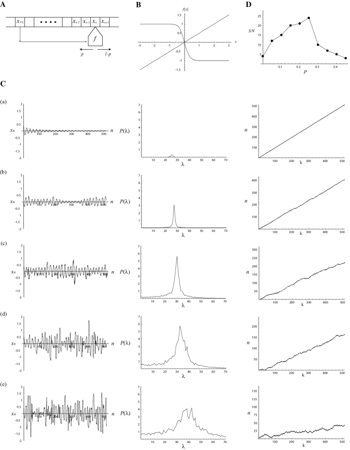
Figure 1: A: A schematic view of the model. B: Dynamical functions $f(x)$ with parameters as examples of simulations presented in this paper. Negative feedback function with parameters $\beta=6$. Straight line has slope of $\alpha=0.5$. C: Dynamics (left) and power spectrum (middle) of delayed dynamical model with stochastic time flow (right). This is an example of the dynamics and associated power spectrum through the simulation of the model given in Eq. (3) with the probability $p$ of stochastic time flow varied. The parameters are set as $\alpha=0.5$, $\beta=6$, $d\delta=0.1$, $\tau=5$ and the stochastic time flow parameter $p$ are set to (a) $p=0$, (b) $p=0.1$, (c) $p=0.25$, (d) $p=0.35$, and (e) $p=0.45$. We used the initial condition that $x_{n}=0.5(n\leq 0)$, and ${n_{0}}=0$. The simulation is performed up to $k=5000$ steps. At that point the values of $x_{n}$ for $0\leq n\leq L$ with $L=512$ are recorded. The 50 averages are taken for the power spectrum on this recorded $x_{n}$. The unit of frequency $\lambda$ is set as ${1\over L}$, and the power $P(\lambda)$ is in arbitrary units. D: The signal to noise ratio ${S\over N}$ at the peak height as a function of the probability $p$ of stochastic time flow. The parameter settings are the same as in C.

We would like to now discuss a couple of points with respect to our model. First, we can view this model as a dynamical model with non-locality and fluctuation on time axis. Both factors are familiar in “space”, but not on time. We may extend this model to include non-locality and fluctuations in the space variable $x$. Proceeding in this way, we have a picture of dynamical systems with non-locality and fluctuations on both the time and space axes. The analytical framework and tools for such a description need to be developed, along with a search for appropriate applications.

Another way might be to extend the path integral formalism. The question of whether this extension bridges to quantum mechanics and/or leads to an alternative understanding of such properties as time-energy uncertainty relations also requires further investigation. Also, there is a theory of elementary particles with a fluctuation of space–time, where the noise term is added to the metrictakano . If we can connect our ideas here to such a theory remains to be seen.

Finally, if these models do capture some aspects of reality, particularly with respect to stochasticity in the time flow, this resonance may be used as an experimental indication for probing fluctuations or stochasticity in time. We have previously proposed “delayed stochastic resonance”ohira-sato , a resonance that results from the interplay of noise and delay. It was theoretically extendedtsimring01 , and recently, the effect was experimentally observed in a solid-sate laser system with a feedback loopmasoller . It is left for the future to see if an analogous experimental test could be developed with respect to stochastic time.

References

- (1) P. Davies, About Time, (Simon and Schuster, New York, 1995).
- (2) S. F. Savitt, Time’s Arrows Today, (Cambridge Univ. Press, Cambridge, 1995).
- (3) P. Busch, “The Time-Energy Uncertainty Relation,” in Time in Quantum Mechanics (J. G. Muga, R. Sala Mayato and I. L. Egusquiza, eds. ) 69-98 (Springer-Verlag, Berlin, 2002).
- (4) M. C. Mackey and L. Glass, Science 197, 287–289 (1977).
- (5) K. L. Cooke and Z. Grossman, J. Math. Anal. and Appl. 86, 592–627 (1982).
- (6) J. G. Milton, et al., J. Theo. Biol. 138, 129–147 (1989).
- (7) T. Ohira and T. Yamane, Phys. Rev. E 61, 1247–1257 (2000).
- (8) T. D. Frank and P. J. Beek, Phys. Rev. E 64, 021917 (2001).
- (9) K. Wiesenfeld, and F. Moss, Nature 373, 33–36 (1995).
- (10) A. R. Bulsara and L. Gammaitoni, Physics Today 49, 39–45 (1996).
- (11) L. Gammaitoni, P. Hänggi, P. Jung, and F. Marchesoni, Rev. Mod. Phys. 70, 223–287 (1998).
- (12) B. McNamara, K. Wiesenfeld and R. Roy, Phys. Rev. Lett. 60, 2626–2629 (1988).
- (13) A. Longtin, A. Bulsara and F. Moss, Phys. Rev. Lett. 67, 656–659 (1991).
- (14) J. J. Collins, C. C. Chow and T. T. Imhoff, Nature 376, 236–238 (1995).
- (15) F. Chapeau-Blondeau, Sign. Process 83, 665–670 (2003).
- (16) I. Y. Lee, X. Liu, B. Kosko and C. Zhou, Nano Letters 3, 1683–1686 (2003).
- (17) L. Glass and M. Mackey, The Rhythms of Life, (Princeton Univ. Press, Princeton, 1988).
- (18) J. L. Cabrera and J. G. Milton, Phys. Rev. Lett. 89 158702 (2002).
- (19) J. L. Cabrera and J. G. Milton, Chaos 14, 691-698 (2004).
- (20) T. Ohira and Y. Sato, Phys. Rev. Lett. 82, 2811–2815 (1999).
- (21) Y. Takano, Prog. Theor. Phys. 26, 304–314 (1961); Y. Takano, ibid, 38 (1967) 1185–1186.
- (22) L.S. Tsimring and A. Pikovsky, Phys. Rev. Lett. 87 250602 (2001).
- (23) C. Masoller, Phys. Rev. Lett. 88 034102 (2002).