Nonstationary Increments, Scaling Distributions, and Variable Diffusion Processes in Financial Markets

Arguably the most important problem in quantitative finance is to understand the nature of stochastic processes that underlie market dynamics. One aspect of the solution to this problem involves determining characteristics of the distribution of fluctuations in returns. Empirical studies conducted over the last decade have reported that they are non-Gaussian, scale in time, and have power-law (or fat) tails mand ; mccAgun ; manAsta ; friApei ; borl . However, because they use sliding interval methods of analysis, these studies implicitly assume that the underlying process has stationary increments. We explicitly show that this assumption is not valid for the Euro-Dollar exchange rate between 1999-2004. In addition, we find that fluctuations in returns of the exchange rate are uncorrelated and scale as power-laws for certain time intervals during each day. This behavior is consistent with a diffusive process with a diffusion coefficient that depends both on the time and the price change. Within scaling regions, we find that sliding interval methods can generate fat-tailed distributions as an artifact, and that the type of scaling reported in many previous studies does not exist.

Our analysis is conducted on one-minute intra-day prices of the Euro-Dollar exchange rate (obtained from Olsen and Associates, Zürich) which is traded 24-hours a day. Let $P(t)$ represent the exchange rate at time $t$ and define the return of the exchange rate as ${\bar{x}}(\tau;t)\equiv\log\left[P(\tau+t)/P(t)\right]$. Here $t$ represents a time during the day and $\tau$ a time increment that is initiated at $t$. The analysis presented below is predicated on the assumption, for which we provide evidence, that the stochastic dynamics of ${\bar{x}}(\tau;t)$ is the same between trading days. Then, we find that the average movement taken over the approximately 1500 trading days during 1999-2004, $\langle{\bar{x}}(\tau;t)\rangle$ nearly vanishes for each value of $t$. A value of $\tau=10\ min$ is used so that the autocorrelations in the signal $P(t)$ have decayed sufficiently. The rest of our analysis is conducted on fluctuations $x(\tau;t)={\bar{x}}(\tau;t)-\langle{\bar{x}}(\tau;t)\rangle$ about the mean.

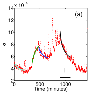
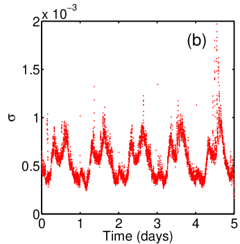
Figure 1: (a) The standard deviation $\sigma(\tau;t)\equiv\sqrt{\langle x(\tau;t)^{2}\rangle}$ of the daily Euro-Dollar exchange as a function of the time of day (in GMT). Here $\tau=10\ min$ to ensure that autocorrelations in $P(t)$ have decayed sufficiently. Our statistical analysis assumes that $x(\tau;t)$ follows the same stochastic process each trading day. The average indicated by the brackets $\langle.\rangle$ is taken over the approximately 1500 trading days between 1999-2004, and the standard error at each point is typically 3%. Note that, if the stochastic dynamics had stationary increments, $\sigma(\tau;t)$ would be constant. Instead, it varies by more than a factor of 3 during the day, thus showing explicitly that the exchange rate has nonstationary increments. Notice also that $\sigma(\tau;t)$ scales in time during several intervals, four of which are highlighted by colored lines that are power-law fits. Our analysis focuses on the interval I shown by the horizontal solid line. (b) The weekly behavior of $\sigma(\tau;t)$ for the same data. Observe that it exhibits an approximate daily periodicity, thereby justifying our assumption of the daily repeatability of the stochastic process underlying the Euro-Dollar exchange rate.

A stochastic process has stationary increments if the distribution of $x(\tau;t)$ is independent of $t$; otherwise, increments are nonstationary. Figure 1(a) shows the behavior of the standard deviation $\sigma(\tau;t)\equiv\sqrt{\langle x(\tau;t)^{2}\rangle}$ of the Euro-Dollar rate as a function of the time of day. If the stochastic increments are stationary, the curve would be flat. Clearly, it is not. Instead $\sigma(\tau;t)$ exhibits complicated nonstationary behavior while changing by more than a factor of 3 during the day.

Our assumption of daily repetition of the stochastic process is validated by conducting a corresponding analysis of fluctuations throughout a trading week galAcal . Figure 1(b) shows the standard deviation of returns averaged over the 300 weeks studied. The approximate daily periodicity of $\sigma(\tau;t)$ is evident, thereby justifying our approach. Similar observations were made on price increaments for Euro-Dollar rate in Ref. galAcal .

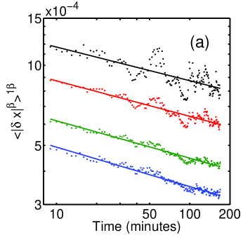
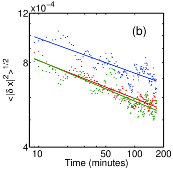
Figure 2: (a) A log-log plot of $\langle x(\tau;t)^{\beta}\rangle^{1/\beta}$ for $\beta=0.5,1.0,2.0$, and $3.0$, demonstrating power law decay $t^{-\eta}$ for each index. Here $t$ is measured in local New York time stating at 9:00AM. The data for $\beta=0.5,1.0,2.0$, and $3.0$, shown in blue, green, red, and black, respectively, have scaling indices (given by the slopes of the solid lines) $\eta=0.15\pm 0.02$, $0.14\pm 0.02$, $0.13\pm 0.04$ and $0.13\pm 0.08$. All of these values are consistent with $\eta\approx 0.15$, and hence a dynamical scaling index of $H=\frac{1}{2}-\eta\approx 0.35$. The error estimates on the exponents are the standard errors from the nonlinear fit including the standard deviations for each time point, but neglecting any correlations between them. (b) The behavior of the standard deviation $\sigma(\tau;t)$ in the interval I during each of the periods 1999-2000 (blue), 2001-2002 (red), and 2003-2004 (green). The scaling index from nonlinear fits for the three data sets are $0.13\pm 0.06$, $0.14\pm 0.04$ and $0.14\pm 0.07$. The near equality of these indices shows that the scaling index is nearly invariant over time.

The standard deviation scales as power-laws with time during several intervals within the day. Power-law fits to the data in some of these intervals are shown by colored lines in Fig. 1(a). We focus our analysis on the time interval I which begins at 9:00 AM New York time and lasts approximately $3$ hours. The data shown in red in Fig. 2(a) shows that the standard deviation within this interval scales like $t^{-\eta}$ where $t$ is measured from the beginning of the interval and the index $\eta=0.13\pm 0.04$. This scaling extends for more than $1.5$ decades in time. Note that the value of $\eta$ is different for the other time intervals during which the standard deviation scales in time. Similar variation in scaling exponents during the day has been reported previously carAcas .

The scaling index within I does not change significantly during the six years studied. This is demonstrated by independently analyzing three two-year periods 1999-2000, 2001-2002, and 2003-2004. Figure 2(b) shows that the scaling index remains nearly unchanged between these two-year periods.

We have also analyzed the behavior of other moments $\langle|x(\tau;t)|^{\beta}\rangle^{1/\beta}$ of the returns. Figure 2(a) shows that each of the moments $\beta=0.5,\ 1.0,\ 2.0$, and $3.0$ also scales as a power-law in time, and furthermore that the scaling index for each of them is consistent with the value of $\eta=0.15$. This nearly uniform scaling of the different moments suggests that the return distribution itself scales in time. Denote the distribution of $x(\tau;t)$ by $W(x,\tau;t)$, where the final argument reiterates that the distribution can depend on the starting time of the interval. In particular, when the increments are nonstationary $W(x,\tau;t)$ depends on $t$. Our scaling anzatz is

$$W(x,\tau;0)=\frac{1}{\tau^{H}}{\cal F}(u)$$ (1)

where $H$ is the scaling index, $u=x/\tau^{H}$ the scaling variable and ${\cal F}$ the scaling function. Note that the scaling anzatz is for a time interval starting from the beginning of I.

In addition to scaling, the stochastic dynamics appears to have no memory. This can be demonstrated by evaluating the auto-correlation function

$$A_{\tau}(t_{1},t_{2})=\frac{\langle x(\tau;t_{1})x(\tau;t_{2})\rangle}{\sigma(\tau;t_{1})\sigma(\tau;t_{2})}.$$

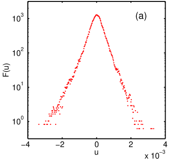
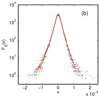
Figure 4: (a) The empirical scaling function ${\cal F}$ for interval I calculated assuming the scaling anzatz Eq. (1) with $H=0.35$ and values of $\tau$ between 10 and 160 minutes. Note that ${\cal F}$ is slightly asymmetric and approximately bi-exponential. Since exponential distributions have finite variance, all assumptions needed for the derivation of Eq. (2) are justified. (b) The empirical sliding interval scaling function ${\cal F}_{S}$ for interval I calculated by scaling collapse of data using the anzatz Eq. (3) for $\tau$ of 10 (blue), 20 (green) and 40 (red) minutes. Note that ${\cal F}_{S}$ has fat-tails.

We find that for $\tau=10$, $A_{\tau}(t_{1},t_{2})=1$ if $t_{1}=t_{2}$, and of the order of $10^{-3}$ when $|t_{1}-t_{2}|\geq 10$. This observation eliminates fractional Brownian motion manAvan as a description for the underlying stochastic dynamics, and strongly indicates that ${\partial W(x,\tau;0)}/{\partial\tau}$ depends only on $x(\tau;0)$ and $\tau$. If, in addition, $W(x,\tau;0)$ has finite variance (see Fig. 4), it has been analytically established that the evolution of $W(x,\tau;0)$ is given by a diffusion equation chan ; gunAmcc

$$\frac{\partial W(x,\tau;0)}{\partial\tau}=\frac{1}{2}\frac{\partial^{2}}{\partial x^{2}}\left(D(x,\tau)W(x,\tau;0)\right),$$ (2)

where $D(x,\tau)$ is the diffusion coefficient. There is no drift term in Eq. (2) because $x(\tau;t)$ has zero mean for all $t$. Note that the stochastic dynamics is completely determined by the diffusion coefficient, which, as shown below, depends on $H$. Hence, $H$ can be considered to be the dynamical scaling index.

Because we have found scaling, consider solutions of the form (1) to Eq. (2). When $H=1/2$, the diffusion coefficient has been shown to be a function of $u$; i.e., $D(x,\tau)={\cal D}(u)$ gunAmcc . If, in addition, ${\cal D}(u)$ is symmetric in $u$, it is related to the scaling function by ${\cal F}(u)=D(u)^{-1}\exp\left(-\int^{u}dy\ y/D(y)\right)$ gunAmcc ; aleAbas . When $H\neq 1/2$, we can “rescale” time intervals by $\tilde{\tau}=\tau^{2H}$ galAcal ; basAgun . In $\tilde{\tau}$, the stochastic process has a scaling index $1/2$ and a diffusion coefficient of the form ${\cal D}(x/\sqrt{\tilde{\tau}})$. Converting back to $\tau$, $D(x,\tau)=2H\tau^{2H-1}{\cal D}(u)$ basAgun .

Statistical analyses of financial markets have often been conducted using sliding interval methods mccAgun ; manAsta ; friApei ; borl ; borl2 ; galAcal ; ghaAbre , which implicitly assume that increments are stationary even if they are not. For example, they compute the distribution $W_{S}(x,\tau)=\langle W(x,\tau;t)\rangle_{t}$, where $\langle.\rangle_{t}$ indicates an average over $t$. Many of these studies have reported that $W_{S}(x,\tau)$ scales as

$$W_{S}(x,\tau)=\frac{1}{\tau^{H_{S}}}{\cal F}_{S}(v),$$ (3)

where $v=x/{\tau^{H_{S}}}$ and $H_{S}\approx 1/2$. It has also been reported that the scaling function ${\cal F}_{S}$ has power-law (or fat) tails friApei ; borl . However, it is important to understand that $W_{S}(x,\tau)$ is a solution of Eq. (2) only when the stochastic process has stationary increments, in which case $H=H_{S}=1/2$. In general, $H_{S}$ and $W_{S}(x,\tau)$ are different from $H$ and $W(x,\tau;0)$. Next, we give an explicit example where this is the case, and, in addition, $W_{S}(x,\tau)$ appears to have fat-tails even though $W(x,\tau;0)$ does not.

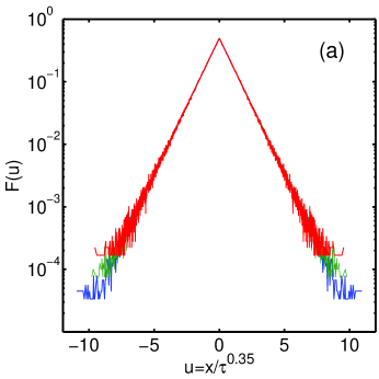
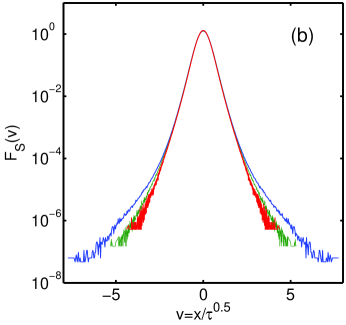
Figure 3: (a) The scaling function of the return distribution ${\cal F}$ calculated from a collapse of data for $\tau=10$ (blue), $100$ (green), and $1000$ (red) units. The results are from a set of 5,000,000 independent stochastic processes with variable diffusion. The scaling index used was $H=0.35$, and the diffusion coefficient was $2Ht^{2H-1}(1+|u|)$. Note that ${\cal F}$ is bi-exponential, as discussed in the text. (b) The sliding interval scaling function ${\cal F}_{S}$ calculated from the same runs. Shown are results for sliding intervals with $\tau=10$ (blue), $100$ (green) and $1000$ (red) units from runs of length $10,000$ units. Unlike ${\cal F}$, it appears to have fat tails. The scaling index used here for which the scaling collapse is achieved is $H_{S}=1/2$ even though the dynamical scaling index is $H=0.35$. Note, however, although the central part of the distribution scales well, the tails do not.

Consider a diffusive process initiated at $x=0$ that has a variable diffusion coefficient $2H\tau^{2H-1}(1+|u|)$. Its distribution has a scaling index $H$ and a scaling function ${\cal F}(u)=\frac{1}{2}\exp(-|u|)$ gunAmcc ; aleAbas . (See the discussion following Eq. (2).) Numerical integration of the stochastic process for $H=0.35$ confirms this claim, see Fig. 3(a). In contrast, $W_{S}(x,\tau)$ calculated from the same data appears to scale with an index $H_{S}=\frac{1}{2}$. Unlike ${\cal F}$ which is bi-exponential, the apparent scaling function ${\cal F}_{S}$ (shown in Fig. 3(b)) has fat-tails. However, a careful analysis reveals that distributions $W_{S}(x,\tau)$ do not scale in the tail region, and hence that ${\cal F}_{S}$ is not well-defined. Differences analogous to those between $H$ and $H_{S}$ have been noted for Lévy processes fogAboh and for the R/S analysis of Tsallis distributions borl2 .

The behavior of $\sigma(\tau;t)$ (Fig. 2(a)) can be calculated for variable diffusion processes. Assuming that $\tau$ is small, Ito calculus gives $\delta x^{2}\equiv x(\tau;t)^{2}=D(x,t)\tau$. Averaging over returns at $t$ gives

$$\langle\delta x^{2}\rangle=\left[\int dxW(x,t;0)D(x,t)\right]\tau.$$ (4)

In a variable diffusion process, $W(x,t;0)=t^{-H}{\cal F}(u)$ and $D(x;t)=2Ht^{2H-1}{\cal D}(u)$; consequently

$$\sqrt{\langle\delta x^{2}\rangle}\sim t^{H-1/2},$$ (5)

independent of the exact form of ${\cal D}(u)$. Results for the Euro-Dollar rate within the interval I (Fig. 2(a)) which showed that $\eta\approx 0.15$ are therefore consistent with a scaling index $H=\frac{1}{2}-\eta\approx 0.35$. Note that, unlike for Lévy processes and fractional Brownian motion, $H<1/2$, and is substantially less than $H_{S}$ reported in previous analyses of the Euro-Dollar exchange rate (between 0.5 and 0.6) galAcal ; ghaAbre ; mulAdac . A general calculation for the moments of a variable diffusion process gives

$$\langle|\delta x|^{\beta}\rangle^{1/\beta}\sim t^{H-1/2},$$ (6)

for all $\beta$, consistent with results shown in Fig. 2(a).

In order to estimate $H_{S}$ for an arbitrary variable diffusion process, we note first that $\langle x(t+\tau;0)^{2}\rangle=\langle x(t;0)^{2}\rangle+\langle x(\tau;t)^{2}\rangle$ for any diffusive process without memory (see Ref.gunAmcc ). Then, using the scaling anzatz (1), setting $c=\int du\ u{\cal F}(u)$, and taking the sliding interval average

$$\langle x(\tau;t)^{2}\rangle_{t}=\langle c(t+\tau)^{2H}-ct^{2H}\rangle_{t}\approx 2Hc\langle t^{2H-1}\rangle_{t}\tau,$$ (7)

where the last approximation is valid when $\tau\ll t$, a condition that is true for most intervals of length $\tau$ in a sliding interval calculation. Hence $\langle x(\tau;t)^{2}\rangle_{t}\sim\tau$. Consequently, $H_{S}=1/2$ regardless of the value of $H$!

Finally, we introduce a method to extract the empirical scaling function ${\cal F}$ from the Euro-Dollar time series. Unfortunately, the available data are insufficient to determine ${\cal F}(u)$ accurately using the usual method of collapsing $W(x,\tau;0)$ for multiple values of $\tau$. However, since we have determined $H(\approx 0.35)$ independently, we can use Eq. (1) for multiple values of $\tau$ in the interval I (i.e., $\tau$ between approximately $10$ and $160$ minutes) to determine ${\cal F}$. The result is shown in Fig. 4(a). Note that the distribution has an approximate bi-exponential form. Since exponential distributions have finite variance, all assumptions needed for the derivation of Eq. (2) are justified. However, it is asymmetric and decays more slowly on the negative side. By contrast, the empirical sliding interval scaling function ${\cal F}_{S}(v)$ for the same time interval is shown in Fig. 4(b). For this case, the scaling collapse is achieved for $H_{S}=1/2$. $F_{S}(v)$ appears to have fat tails, consistent with previous reports mulAdac ; borl . However, in light of the example discussed earlier and the fact that $H\neq 1/2$, it is unlikely that ${\cal F}_{S}$ is well-defined for this financial market data within the interval I.

Variable diffusion processes exhibit another signature (stylized fact) of market fluctuations. Although their autocorrelation vanishes, a large fluctuation will typically produce a large value of $|x|$, and hence a return with a large diffusion coefficient. Consequently, a large fluctuation is likely to be followed by additional large fluctuations whose signs are uncorrelated to the first gunAmcc . As a result, the autocorrelation function for the signal $|x(\tau;t)|$ (or for the signal $x(\tau;t)^{2}$) will decay slowly in $t$. Such behavior, referred to as the “clustering of volatility” is seen in the Euro-Dollar exchange rate and has been reported in empirical studies of other financial markets conApot ; heyAyan ; heyAleo .

The analysis given here applies to stochastic dynamics of a single scaling interval. However, the daily fluctuations in the Euro-Dollar rate are a combination of scaling intervals with distinct scaling indices, and possibly regions with no scaling. We have not yet determined how to extend our analysis beyond a single scaling region. Bacuase of this, it is not clear how to interpret the distributions over intervals longer than a scaling region, including inter-day data.

We have shown that stochastic fluctuations in the Euro-Dollar rate have uncorrelated nonstationary increments during the course of a trading day, and that there are intervals during which their absolute moments scale like a power-law in time. The stochastic dynamics during these scaling intervals can be described by a diffusion process with variable diffusion coefficient. We have also shown that sliding interval analysis of variable diffusion processes can give an incorrect scaling exponent and in addition can give scaling functions with fat-tails even when the underlying dynamics do not have them. Indeed, this appears to be the case within the interval I.

The authors would like to thank A. A. Alejandro-Quinones for discussions. They also acknowledge support from the Institute for Space Science Operations (KEB, GHG) and the NSF through grants DMR-0406323 (KEB), DMR-0427938 (KEB) and DMS-0607345 (GHG).

References

- (1) B. B. Mandelbrot, The Variation of Certain Speculative Prices, J. Bus. 36, 394 (1963).
- (2) J. L. McCauley and G. H. Gunaratne, An Empirical Model of Volatility Returns and Options Pricing, Physica A 329, 170 (2003).
- (3) R. N. Mantegna and H. E. Stanley, Scaling Behavior in the Dynamics of an Economic Index, Nature 376, 46 (1995); Turbulence in Financial Markets, Nature 383, 587 (1996).
- (4) R. Friedrich, J. Peinke, and Ch. Renner, How to Quantify Deterministic and Random Influences on the Statistics of the Foreign Exchange Market, Phys. Rev. Lett. 84, 5224 (2000).
- (5) L. Borland, A Theory of Non-Gaussian Option Pricing, Quan. Finance 2, 415 (2002).
- (6) S. Galluccio, G. Caldarelli, M. Marsili, and Y. C. Zhang, Scaling in Currency Exchange, Physica A 245, 423 (1997).
- (7) A. Carbone, G. Castelli, and H. E. Stanley, Time-dependent Hurst Exponents in Financial Time Series, Physica A 344, 267 (2004).
- (8) B. Mandlebrot and J. W. van Ness, Fractional Brownian Motion, Fractional Noise and Applications, SIAM Rev. 10, 422 (1968).
- (9) G. H. Gunaratne, J. L. McCauley, M. Nicole, and A. Török. Variable Step Random Walks and Self-Similar Distributions, J. Stat. Phys. 121, 887 (2005).
- (10) S. Chandrasekhar, Stochastic Problems in Physics and Astronomy, Rev. Mod. Phys., 15, 1 (1943).
- (11) A. A. Alejandro-Quinones, K. E. Bassler, M. Field, J. L. McCauley, M. Nicol, I. Timofeyev, A. Török, and G. H. Gunaratne, A Theory of Fluctuations in Stock Prices, Physica A 363, 383 (2006).
- (12) K. E. Bassler, G. H. Gunaratne, and J. L. McCauley, Markov Processes, Hurst Exponents, and Nonlinear Diffusion Equations with Applications to Finance, Physica A, 369, 343 (2006).
- (13) L. Borland, Microscopic Dynamics of the Nonlinear Fokker-Planck Equation: A Phenomenological Model, Phys. Rev. E 57, 6634 (1998).
- (14) S. Ghashghaie, W. Breymann, J. Peinke, P. Talkner, and Y. Dodge, Turbulent Cascades in Foreign Exchange Markets, Nature 381, 767 (1996).
- (15) H. C. Fogedby, T. Bohr, and H. J. Jensen, Fluctuations in a Lévy Flight Gas, J. Stat. Phys. 66, 583 (1992).
- (16) U. A. Müller, M. M. Dacorogna, R. B. Olsen, O. V. Pictet, M. Schwarz, and C. Morgenegg, Statistical Study of Foreign Exchange Rates, Empirical Evidence of a Price Change Scaling Law, and Inter-day Analysis, J. Bank. Fin. 14, 1189 (1990).
- (17) R. Cont, M. Potters, and J.-P. Bouchard, Scaling in Stock Market Data: Stable Laws and Beyond, in ”Scale Invariance and Beyond”, eds. B. Dubrulle, F. Graner, and D. Sornette, Springer, Berlin, 1997.
- (18) C. C. Heyde and Y. Yang, On Defining Long Range Dependence, J. Appl. Prob. 34, 939 (1997).
- (19) C. C. Heyde and N. N. Leonenko, Student Processes, Adv. Appl. Prob. 37, 342 (2005).
- (20) M. Couillard and M. Davison, A Comment on Measuring the Hurst exponent of Financial Time Series, Physica A 348, 404 (2005).