Equilibrium configurations of tripolar charges

Abstract

It is shown that an ensemble of particles with tripolar (colour) charges will necessarily cohere in a hierarchy of structures, from simple clusters and strings to complex aggregates and cyclic molecule-like structures. The basic combinatoric rule remains essentially the same on different levels of the hierarchy, thus leading to a pattern of resemblance between different levels. The number of primitive charges in each structure is determined by the symmetry of the combined effective potential of this structure. The outlined scheme can serve as a framework for building a model of composite fundamental fermions. PACS: 89.75.Fb, 36.90.+f, 12.60.RC, 12.15.Ff.

1 Introduction

It is known that the structures of important objects that physicists study, like stars, galaxies, molecules, atoms, nucleons, and some particles, are equilibrium states between opposing forces of nature. Equilibrium potentials are broadly used for modelling molecules [1, 2], vortices in superconductors [3, 4], metal structures [5], and even granular materials [6]. Realistic interactions between molecules are known to have always attractive and repulsive components, due to the fact that solids and liquids have the property of cohesion but, at the same time, do not collapse to a point under the action of these forces. Such systems are modelled with potentials that comprise a repulsive inner and an attractive outer region (or vice versa). A similar approach is often used in biochemistry [7], colloid chemistry [8], in material sciences [9], and many other branches of physics and chemistry.

In condensed matter, the interactions between neutral atoms are described by the equilibrium Lennard-Jones and Morse potentials. The electron cloud of a neutral atom fluctuates about the positively charged nucleus. The fluctuations in neighbouring atoms become correlated, inducing attractive dipole-dipole interactions. The equilibrium distance between two proximal atomic centres is determined by a trade-off between this attractive (van der Waals) dispersion force and a core-repulsion force that reflects electrostatic repulsion and the Pauli exclusion principle.

For simplicity, the Lennard-Jones forces are typically modelled as effectively pair-wise additive, and the velocities and positions of atoms are calculated by numerical methods as a multi-body problem of mechanics. The effective potential in these systems is represented as a sum of one-body, two-body and three-body components. The task can be simplified by coupling two-body and higher multi-atom correlations in one model [10]. The central idea is that in real systems, the strength of each bond depends on the local environment, i.e. an atom with many neighbours forms weaker bonds than an atom with few neighbours. Then, one can use a pair potential, the strength of which depends on the environment (screened potential in the Morse form). This is related to the exponential decay dependence of the electronic density and is usually written as:

$$\begin{split}&\sum_{i}E_{i}=\frac{1}{2}\sum_{i\neq j}V_{ij},\\ &V_{ij}(r_{ij})=F_{C}(r_{ij})[F_{\ominus}(r_{ij})+b_{ij}F_{\oplus}(r_{ij})],\end{split}$$ (1)

where the potential energy is resolved into a site energy $E_{i}$ and a bonding energy $V_{ij}$ between the particles $i$ and $j$; $r_{ij}$ is the distance between the particles (atoms); $F_{\ominus}$ and $F_{\oplus}$ are the attractive and repulsive pair potentials:

$$\begin{split}&F_{\ominus}(r)=~{}~{}a_{\ominus}\exp{(-\lambda_{\ominus}r)},\\ &F_{\oplus}(r)=-a_{\oplus}\exp{(-\lambda_{\oplus}r)},\end{split}$$ (2)

and $F_{C}$ is a cut-off function. The strengths ($a_{\ominus}$ and $a_{\oplus}$) and the range of each bond depend on the local environment and are reduced when the number of neighbours is relatively high. This dependency is expressed by $b_{ij}$, which can enhance or diminish the repulsive force relative to the attractive force, according to the environment.

In this paper we shall apply a similar approach to the structures with tripolar charges, taking into account the possibility of attractive and repulsive forces being different by their nature, rather than both having an electrostatic origin. Indeed, in hadron and quark systems the attractive and repulsive forces correspond to the strong (tripolar) interactions described by quantum chromodynamics [11]. Currently the attention of nuclear-physicists is focused primarily on the strong interactions in quark-gluon plasma and multi-quark systems. Some results of these studies, such as the estimation of the top-quark mass [12] and prediction of pentaquarks [13], are confirmed by observations [14, 15, 16], thus showing that the basic features of quantum chromodynamics are consistent with the subnucleonic reality.

However, despite numerous publications on tripolar interactions, to date little attention has been paid to the fact that the strong and electric charges can be modelled by two-component equilibrium fields, by analogy with molecular and condensed matter physics. This approach can effectively yield new results. For example, the phenomenology of the hydrogen molecule (which is not yet well-understood) has been recently explained by introducing an attractive short-range Hulten (hadronic) potential between electrons, in addition to their conventional Coulomb repulsive potential [17].

Although the strong force per se manifests both its attractive and repulsive nature [18], we shall include in our model both strong and electric field components. For the sake of simplicity we shall use identical particles, all having the same (unit) mass and charge.

The tripolar fields are usually labelled with three primary colours, which is also convenient for visualisation purposes [19]. For instance, a colour-neutral system (unaffected by any colour charge) can be represented (both mathematically and graphically) as a superposition of three complementary colours in equal proportions (usually red, green and blue). This can be viewed as a “white” colour-charge (or “black”, if the magnitudes of all three colours are mutually cancelled).

2 Basic potential

Let us consider a spherically symmetric equilibrium potential of a primitive particle P with no properties, save its basic symmetry of SU(3)/U(1)-type. That is, this particle has both electric and colour (unit) charges. We shall regard a field $F(\rho)$ associated with such a particle as a superposition of two components, one attractive, $F_{\ominus}(\rho)$, and another repulsive, $F_{\oplus}(\rho)$, satisfying the following conditions:

$$F(0)=F^{\prime}(0)=0,$$ (3)

$$\exists\rho_{\circ}>0:\hskip 5.69046ptF_{\oplus}(\rho_{\circ})=-F_{\ominus}(\rho_{\circ})$$ (4)

(where $\rho$ is the radial coordinate). We also assume the applicability of the least-action principle to the field $F$. The condition (4) implies that the components of the field cancel each other in the vicinity of some distance $\rho_{\circ}$, corresponding to equilibrium in a two-particle system.

We suppose that both components of the field $F$ are closely related to each other (because they are underlied by the same source – the primitive particle P). This means that any local changes in one component of the field are reflected in the other, which would result in suppression of possible fluctuations in an equilibrium system composed of a few primitive particles.

In order to represent the colour-neutral systems we have to introduce a special notation for three colour polarities, complementary to each other. Let the vectors $\bf{r}$, $\bf{g}$, and $\bf{b}$ be the signatures of the three primary colour charges (red, green and blue), such that the “white” colour is

$$\mathbf{w}=\mathbf{r}+\mathbf{g}+\mathbf{b},$$ (5)

where $\mathbf{w}$ is the diagonal of a unit matrix. In order to satisfy (5), the $\bf{rgb}$-vectors could have the following components:

$$\begin{split}\mathbf{r}&=(-1,+1,+1)^{\intercal}\\ \mathbf{g}&=(+1,-1,+1)^{\intercal}\\ \mathbf{b}&=(+1,+1,-1)^{\intercal}.\end{split}$$ (6)

In the case of a system with mutually cancelled colour charges we can write

$$\mathbf{r}+\mathbf{g}+\mathbf{b}-\mathbf{w}=\mathbf{0},$$ (7)

which would correspond to a colour-neutral system with null electric charge.

With this notation, the field $F_{i}(\rho)$ of a particle ${\sf P}_{i}$ that has a colour $\mathbf{c}_{i}\in\{\mathbf{r},\mathbf{g},\mathbf{b}\}$ can be written as

$$\mathbf{F}_{i}(\rho)=\mathbf{c}_{i}F_{\oplus}(\rho)+(\mathbf{c}_{i}-\mathbf{w}/3)F_{\ominus}(\rho).$$ (8)

In particular, in a system with $N=3$ complementary colour charges (say, $\mathbf{c}_{1}=\mathbf{r}$, $\mathbf{c}_{2}=\mathbf{g}$, $\mathbf{c}_{3}=\mathbf{b}$), the superposition of the fields $F_{i}$ will contain only the terms with $F_{\oplus}$:

$$\sum_{i=1}^{3}\mathbf{F}_{i}=\mathbf{w}F_{\oplus},$$

because

$$\sum_{i=1}^{3}(\mathbf{c}_{i}-\mathbf{w}/3)=\mathbf{0},$$

and the terms with $F_{\ominus}$ are mutually cancelled.

As a simple example of the split equilibrium field one can consider the field with the following components

$$F_{\ominus}=F_{0}(\rho),\hskip 11.38092ptF_{\oplus}=F^{\prime}_{0}(\rho),$$ (9)

where

$$F_{0}(\rho)=s_{ij}a_{0}\exp(-\lambda_{0}\rho^{-1}).$$ (10)

The derivative in (9) is taken with respect to the radial coordinate, $\rho$. The coefficient $s_{ij}=\pm 1$ (signature) in (10) accounts for the sign of the interaction (repulsion or attraction) between two colour-charged particles, say, ${\sf P}_{i}$ and ${\sf P}_{j}$. For the sake of simplicity let the strength and range coefficients be normalised to unity ($a_{0}=\lambda_{0}=1$). The functions $F_{\ominus}(\rho)$ and $F_{\oplus}(\rho)$, and the corresponding combined potential $V(\rho)$ are plotted in Fig.1 (for $s_{ij}=-1$), where the unit distance, $\rho_{\circ}$, corresponds to (4).

Figure 1: Components $F_{\ominus}$ and $F_{\oplus}$ of the equilibrium field $F$, and the corresponding potential, $V(\rho)$, for the signature $s_{ij}=-1$ in (10).

3 Colour dipoles and tripoles

Obviously, the simplest structures allowed by the tripolar field are the monopoles, dipoles and tripoles, unlike the conventional bipolar (electric) field, which allows only the monopoles and dipoles. Here we shall consider the colour dipoles and tripoles. The potentials shown in Fig.1 correspond to a pair of like-charged ($F_{\oplus}$ – repulsive) primitive particles with unlike-colours ($F_{\ominus}$ – attractive), which constitute a charged colour dipole ${\sf C}^{2}_{ij}={\sf P}_{i}+{\sf P}_{j}$. Here the indices $i$ and $j$ label the colour charges of the dipole’s constituents: $i,j\in\{r,g,b\}$, $i\neq j$; the upper index “2” stands for the number of particles involved. As with any other dipole, the components of ${\sf C}^{2}_{ij}$ will oscillate near an equilibrium point at $\rho=\rho_{\circ}$, where the potential $V(\rho)$ has a minimum. The two components of $F$ are approximately antisymmetric in the vicinity of the origin, which would lead to suppression of these oscillations. Then, the estimation of the ground-state energies (masses) of such a system will be simplified because one can neglect the oscillatory energy of ${\sf P}_{i}$ and ${\sf P}_{j}$ and, to a first-order approximation, compute the mass of the system as a sum of the masses of its constituents.

The existence of a second stationary point in the potential – at the origin – means that the dipole’s constituents, if confined within a very small volume, can be found in a spherically-symmetric superposition state at $\rho=0$. But this state is unstable and its spherical symmetry can be spontaneously broken, with $\rho\rightarrow\rho_{\circ}$, resulting in the polarisation of the system. This also breaks another fundamental symmetry – that of scale invariance.

Given the field $F(\rho)$ being split in two components, the rest energy of the particle P,

$$-\int\limits_{0}^{\infty}F(\rho)d\rho,$$

can be resolved into two parts, containing

$$\int\limits_{0}^{\infty}F_{\ominus}(\rho)d\rho\hskip 11.38092pt\text{and}\hskip 11.38092pt\int\limits_{0}^{\infty}F_{\oplus}(\rho)d\rho,$$ (11)

which can be viewed as two mass terms, $\tilde{m}_{\sf P}$ and $m_{\sf P}$, respectively. With (10) normalised to unity, the second term, $m_{\sf P}$, is also a unity (let us denote this unit mass as $m_{\circ}$). But the first integral in (11) diverges ($\tilde{m}_{\sf P}=\infty$), implying that within the chosen approach the primitive colour charges cannot exist in free states because of their infinite energies.

    

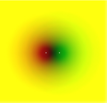
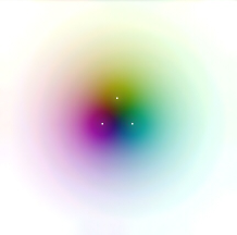
Figure 2: (a): The field of the colour dipole, ${\sf C}^{2}_{ij}$, is deficient in one colour, in this case blue, which is seen as an excess of the complementary colour (yellow) around the dipole. (b): The field of the $\triangle$-shaped (charged) tripole ${\sf C}^{3}$ in its equatorial plane. At some distance from the tripole its field is colourless (unaffected by any colour charge). The white dots mark the centres of the dipole and tripole constituents.

The same is valid for the case of the colour-dipole, ${\sf C}^{2}_{ij}$, which has only two of three possible colour fields $F_{\ominus}$ that cancel one another. This is illustrated in Fig.2(a) where the dipole is shown for the colours $\mathbf{c}_{i}=\mathbf{r}$ and $\mathbf{c}_{j}=\mathbf{g}$. The deficient (diverging) colour, complementary to the other two, is blue, which is seen as an excess of yellow (white minus blue). Similar chromofields were discussed in [20], based on the Gaussian dielectric function and chiral chromodielectric model [21, 22], and also in [23].

Returning to the particle (inertial) masses, we must note that in the current literature there is no agreement as to the origin of mass or inertia. In the Standard Model of particle physics, the initially massless fundamental particles acquire their masses through interactions with the Higgs field. This is currently not yet supported by observations, and in this paper we are free to adhere to a different view that mass is a purely electromagnetic phenomenon. In the simplified approach of this paper we shall not be considering any other forces rather than the electrostatic force caused by the equilibrium field $F(\rho)$. However, contrary to the conventional Coulomb gauge, we shall not regard the field $F(\rho)$ as acting instantaneously at a distance because this would be incompatible with the causality principle. It is more sensible to suggest that the field flow rate is not infinite. Then, there will be a time delay between the action on one part of a system and the response from its another part. This can be viewed as inertia of the system, and the mass of such a system can be regarded as a measure of this delayed response to the external action. That is, the more components of the system are to respond to this action and the more mutually interacting components contribute to that response, the higher mass should be assigned to this system.

To formalise the calculation of masses, we shall represent the discharge of the primitive colour particle with the use of auxiliary $3\times 3$ singular matrices  ${\begin{turn}{-180.0}\raisebox{-7.19025pt}{\begin{turn}{-180.0}\raisebox{-7.19025pt}{\sf P}\end{turn}}\end{turn}}\raisebox{6.45831pt}{\tiny\begin{turn}{-180.0}\raisebox{-3.59512pt}{\begin{turn}{-180.0}\raisebox{-3.59512pt}{$\pm$}\end{turn}}\end{turn}}\hskip 4.30554pt~{}_{i}$ containing the following elements:

$${}^{\pm}p^{i}_{jk}=\pm\delta^{i}_{j}(-1)^{\delta^{k}_{j}},$$ (12)

where $\delta^{i}_{j}$ is the Kronecker delta-function; the $\pm$-signs correspond to the sign of the charge; and the index $i$ stands for the colour ($i=1,2,3$ or red, green and blue). The diverging components of the field can be represented by reciprocal elements:

$$\tilde{p}_{jk}=p_{jk}^{-1}.$$

Then, we can define the charges and masses of the primitive particles by summation of these matrix elements:

$$q_{\sf P}=\mathbf{w}^{\intercal}{\sf P}\mathbf{w}\hskip 2.84544pt,\hskip 8.5359pt\tilde{q}_{\sf P}=\mathbf{w}^{\intercal}\tilde{\sf P}\mathbf{w}$$ (13)

and

$$m_{\sf P}=\lvert\mathbf{w}^{\intercal}{\sf P}\mathbf{w}\rvert\hskip 2.84544pt,\hskip 8.5359pt\tilde{m}_{\sf P}=\lvert\mathbf{w}^{\intercal}\tilde{\sf P}\mathbf{w}\rvert$$ (14)

($\tilde{q}_{P}$ and $\tilde{m}_{P}$ diverge). The same matrices P can be used when calculating the signature $s_{ij}$ in (10) for the colours $i$ and $j$:

$$s_{ij}=-\mathbf{w}^{\intercal}{\sf P}_{i}{\sf P}_{j}\mathbf{w}.$$ (15)

In this notation the positively charged dipole   C $+$    $2$   (Fig.2a) can be represented as a sum of two matrices,  ${\begin{turn}{-180.0}\raisebox{-7.19025pt}{\begin{turn}{-180.0}\raisebox{-7.19025pt}{\sf P}\end{turn}}\end{turn}}\raisebox{6.45831pt}{\tiny\begin{turn}{-180.0}\raisebox{-3.59512pt}{\begin{turn}{-180.0}\raisebox{-3.59512pt}{$+$}\end{turn}}\end{turn}}\hskip 4.30554pt_{1}$ and  ${\begin{turn}{-180.0}\raisebox{-7.19025pt}{\begin{turn}{-180.0}\raisebox{-7.19025pt}{\sf P}\end{turn}}\end{turn}}\raisebox{6.45831pt}{\tiny\begin{turn}{-180.0}\raisebox{-3.59512pt}{\begin{turn}{-180.0}\raisebox{-3.59512pt}{$+$}\end{turn}}\end{turn}}\hskip 4.30554pt_{2}$:

$${{\begin{turn}{-180.0}\raisebox{-7.19025pt}{\begin{turn}{-180.0}\raisebox{-7.19025pt}{\sf C}\end{turn}}\end{turn}}\raisebox{4.73611pt}{\tiny\begin{turn}{-180.0}\raisebox{-3.59512pt}{\begin{turn}{-180.0}\raisebox{-3.59512pt}{$+$}\end{turn}}\end{turn} \hskip 2.15277pt{\scriptsize\begin{turn}{-180.0}\raisebox{-5.03317pt}{\begin{turn}{-180.0}\raisebox{-5.03317pt}{$2$}\end{turn}}\end{turn}}}}={\begin{turn}{-180.0}\raisebox{-7.19025pt}{\begin{turn}{-180.0}\raisebox{-7.19025pt}{\sf P}\end{turn}}\end{turn}}\raisebox{6.45831pt}{\tiny\begin{turn}{-180.0}\raisebox{-3.59512pt}{\begin{turn}{-180.0}\raisebox{-3.59512pt}{$+$}\end{turn}}\end{turn}}\hskip 4.30554pt_{1}+{\begin{turn}{-180.0}\raisebox{-7.19025pt}{\begin{turn}{-180.0}\raisebox{-7.19025pt}{\sf P}\end{turn}}\end{turn}}\raisebox{6.45831pt}{\tiny\begin{turn}{-180.0}\raisebox{-3.59512pt}{\begin{turn}{-180.0}\raisebox{-3.59512pt}{$+$}\end{turn}}\end{turn}}\hskip 4.30554pt_{2}=\begin{pmatrix}-1&+1&+1\\ +1&-1&+1\\ 0&0&0\end{pmatrix},$$ (16)

with $q_{{\sf C}^{2}}=+2~{}[q_{\circ}]$. If two components of the dipole are oppositely charged:

$${{\begin{turn}{-180.0}\raisebox{-7.19025pt}{\begin{turn}{-180.0}\raisebox{-7.19025pt}{\sf C}\end{turn}}\end{turn}}\raisebox{4.73611pt}{\tiny\begin{turn}{-180.0}\raisebox{-3.59512pt}{\begin{turn}{-180.0}\raisebox{-3.59512pt}{$\circ$}\end{turn}}\end{turn} \hskip 2.36806pt{\scriptsize\begin{turn}{-180.0}\raisebox{-5.03317pt}{\begin{turn}{-180.0}\raisebox{-5.03317pt}{$2$}\end{turn}}\end{turn}}}}={\begin{turn}{-180.0}\raisebox{-7.19025pt}{\begin{turn}{-180.0}\raisebox{-7.19025pt}{\sf P}\end{turn}}\end{turn}}\raisebox{6.45831pt}{\tiny\begin{turn}{-180.0}\raisebox{-3.59512pt}{\begin{turn}{-180.0}\raisebox{-3.59512pt}{$+$}\end{turn}}\end{turn}}\hskip 4.30554pt_{1}+{\begin{turn}{-180.0}\raisebox{-7.19025pt}{\begin{turn}{-180.0}\raisebox{-7.19025pt}{\sf P}\end{turn}}\end{turn}}\raisebox{6.45831pt}{\tiny\begin{turn}{-180.0}\raisebox{-3.59512pt}{\begin{turn}{-180.0}\raisebox{-3.59512pt}{$-$}\end{turn}}\end{turn}}\hskip 4.30554pt_{2}~{}$$ (17)

(of whatever colour combination), then their electric fields cancel each other:

$$q_{{\hskip 2.1097pt{\scriptsize\begin{turn}{-180.0}\raisebox{-5.03317pt}{\begin{turn}{-180.0}\raisebox{-5.03317pt}{\sf C}\end{turn}}\end{turn}}\raisebox{2.1097pt}{\tiny\begin{turn}{-180.0}\raisebox{-3.59512pt}{\begin{turn}{-180.0}\raisebox{-3.59512pt}{$\circ$}\end{turn}}\end{turn} {\tiny\begin{turn}{-180.0}\raisebox{-3.59512pt}{\begin{turn}{-180.0}\raisebox{-3.59512pt}{$2$}\end{turn}}\end{turn}}}}}=0$$ (18)

implying also a negligibly small mass of this neutral dipole. Of course, the complete cancellation of the fields is possible only if the centres of both charges coincide; otherwise, the system is polarised (as with any dipole). The degree of polarisation would depend on the distance between the components. Let us define the mass of a system containing, say, $N$ particles, as proportional to the number of these particles, wherever their field flow rates are not cancelled. For this purpose, we shall consider (to a first-order approximation) the total field flow rate, $v_{N}$, of such a system as a superposition of the individual volume flow rates of its $N$ components. Then, the total mass can be calculated as the number of particles, $N$, times the normalised to unity field flow rate $v_{N}$:

$$m_{N}=\lvert Nv_{N}\rvert.$$ (19)

Here $v_{N}$ is computed recursively as a (Lorentz additive) superposition of the individual flow rates, $v_{i}$:

$$v_{i}=\frac{q_{i}+v_{i-1}}{1+\lvert q_{i}v_{i-1}\rvert},$$ (20)

where $i=2,\dots,N$; and $v_{1}=q_{1}$. The normalisation condition (20) expresses the common fact that the superposition flow rate of, say, two antiparallel flows ($\uparrow\downarrow$) with equal rate magnitudes $\lvert\mathbf{v}_{\uparrow}\rvert=\lvert\mathbf{v}_{\downarrow}\rvert=v$ vanishes ($v_{\uparrow\downarrow}=0$), whereas, in the case of parallel flows ($\uparrow\uparrow$) it cannot exceed the magnitudes of the individual flow rates ($v_{\uparrow\uparrow}\leq v$). With this notation, the mass of, for instance, the charged colour dipole will be:

$$m_{\hskip 2.1097pt{\scriptsize\begin{turn}{-180.0}\raisebox{-5.03317pt}{\begin{turn}{-180.0}\raisebox{-5.03317pt}{\sf C}\end{turn}}\end{turn}}\raisebox{2.1097pt}{\tiny\begin{turn}{-180.0}\raisebox{-3.59512pt}{\begin{turn}{-180.0}\raisebox{-3.59512pt}{$+$}\end{turn}}\end{turn} {\tiny\begin{turn}{-180.0}\raisebox{-3.59512pt}{\begin{turn}{-180.0}\raisebox{-3.59512pt}{$2$}\end{turn}}\end{turn}}}}\approx 2,\hskip 5.69046pt\tilde{m}_{\hskip 2.1097pt{\scriptsize\begin{turn}{-180.0}\raisebox{-5.03317pt}{\begin{turn}{-180.0}\raisebox{-5.03317pt}{\sf C}\end{turn}}\end{turn}}\raisebox{2.1097pt}{\tiny\begin{turn}{-180.0}\raisebox{-3.59512pt}{\begin{turn}{-180.0}\raisebox{-3.59512pt}{$+$}\end{turn}}\end{turn} {\tiny\begin{turn}{-180.0}\raisebox{-3.59512pt}{\begin{turn}{-180.0}\raisebox{-3.59512pt}{$2$}\end{turn}}\end{turn}}}}=\infty.$$ (21)

The neutral colour dipole will be massless:

$$m_{{\hskip 2.1097pt{\scriptsize\begin{turn}{-180.0}\raisebox{-5.03317pt}{\begin{turn}{-180.0}\raisebox{-5.03317pt}{\sf C}\end{turn}}\end{turn}}\raisebox{2.1097pt}{\tiny\begin{turn}{-180.0}\raisebox{-3.59512pt}{\begin{turn}{-180.0}\raisebox{-3.59512pt}{$\circ$}\end{turn}}\end{turn} {\tiny\begin{turn}{-180.0}\raisebox{-3.59512pt}{\begin{turn}{-180.0}\raisebox{-3.59512pt}{$2$}\end{turn}}\end{turn}}}}}\approx 0$$ (22)

but still

$$\tilde{m}_{{\hskip 2.1097pt{\scriptsize\begin{turn}{-180.0}\raisebox{-5.03317pt}{\begin{turn}{-180.0}\raisebox{-5.03317pt}{\sf C}\end{turn}}\end{turn}}\raisebox{2.1097pt}{\tiny\begin{turn}{-180.0}\raisebox{-3.59512pt}{\begin{turn}{-180.0}\raisebox{-3.59512pt}{$\circ$}\end{turn}}\end{turn} {\tiny\begin{turn}{-180.0}\raisebox{-3.59512pt}{\begin{turn}{-180.0}\raisebox{-3.59512pt}{$2$}\end{turn}}\end{turn}}}}}=\infty$$ (23)

due to the null-elements in the matrix C $\circ$    $2$   (the dipole lacks, at least, one colour charge to make it colour-neutral). The infinities in (21) and (23) imply that neither C $+$    $2$   nor C $\circ$    $2$   can exist in free states. Of course, the flow rate of the electric field of the neutral dipole (and its corresponding mass) is cancelled only approximately (as with any dipole) because the centres of its constituents do not coincide. In an ensemble of a large number of neutral dipoles C $\circ$    $2$  , not only electric but all the chromatic components of the field can be cancelled (statistically).

Obviously, three complementary colour charges will tend to cohere and form a $\triangle$-shaped structure with the distance $\rho_{\circ}$ (of equilibrium) between its components. Thus, by completing the set of colour-charges in the charged dipole (adding, for example, the blue-charged component to the system C $+$    $2$   shown in Fig.2a) one would obtain a colour-neutral (but electrically charged) $\triangle$-shaped tripole:

$${\sf C}^{3}:=[^{~{}g}_{r~{}b}]={\begin{turn}{-180.0}\raisebox{-7.19025pt}{\begin{turn}{-180.0}\raisebox{-7.19025pt}{$\triangle$}\end{turn}}\end{turn}}\raisebox{0.43057pt}{\tiny\begin{turn}{-180.0}\raisebox{-3.59512pt}{\begin{turn}{-180.0}\raisebox{-3.59512pt}{$\blacktriangle$}\end{turn}}\end{turn}}\hskip 0.86108pt~{}~{}.$$ (24)

Hereafter, we shall use the above triangular notation in the structural diagrams representing different tripole combinations (one must not mistake these diagrams for algebraic equations). The marked vertex of the triangle in (24) indicates one of the colour-charges, say, red, to visualise (in the structural diagrams) possible rotations of tripoles with respect to each other. The positively charged $\triangle$-shaped tripole ( C $+$    $3$   or $\triangle$ $+$  ), which can be written in the matrix notation as

$${\begin{turn}{-180.0}\raisebox{-7.19025pt}{\begin{turn}{-180.0}\raisebox{-7.19025pt}{\sf C}\end{turn}}\end{turn}}\raisebox{4.73611pt}{\tiny\begin{turn}{-180.0}\raisebox{-3.59512pt}{\begin{turn}{-180.0}\raisebox{-3.59512pt}{$+$}\end{turn}}\end{turn} \hskip 2.15277pt{\scriptsize\begin{turn}{-180.0}\raisebox{-5.03317pt}{\begin{turn}{-180.0}\raisebox{-5.03317pt}{$3$}\end{turn}}\end{turn}}}={\begin{turn}{-180.0}\raisebox{-7.19025pt}{\begin{turn}{-180.0}\raisebox{-7.19025pt}{\sf P}\end{turn}}\end{turn}}\raisebox{6.45831pt}{\tiny\begin{turn}{-180.0}\raisebox{-3.59512pt}{\begin{turn}{-180.0}\raisebox{-3.59512pt}{$+$}\end{turn}}\end{turn}}\hskip 4.30554pt_{1}+{\begin{turn}{-180.0}\raisebox{-7.19025pt}{\begin{turn}{-180.0}\raisebox{-7.19025pt}{\sf P}\end{turn}}\end{turn}}\raisebox{6.45831pt}{\tiny\begin{turn}{-180.0}\raisebox{-3.59512pt}{\begin{turn}{-180.0}\raisebox{-3.59512pt}{$+$}\end{turn}}\end{turn}}\hskip 4.30554pt_{2}+{\begin{turn}{-180.0}\raisebox{-7.19025pt}{\begin{turn}{-180.0}\raisebox{-7.19025pt}{\sf P}\end{turn}}\end{turn}}\raisebox{6.45831pt}{\tiny\begin{turn}{-180.0}\raisebox{-3.59512pt}{\begin{turn}{-180.0}\raisebox{-3.59512pt}{$+$}\end{turn}}\end{turn}}\hskip 4.30554pt_{3}=\begin{pmatrix}-1&+1&+1\\ +1&-1&+1\\ +1&+1&-1\end{pmatrix}~{},$$

is colour-neutral at infinity but colour-polarised in the vicinity of its constituents (see Fig.2b). Both $m$ and $\tilde{m}$ of ${\sf C}^{3}$ are finite:

$$m_{\triangle}=\tilde{m}_{\triangle}=3~{}[m_{\circ}],$$

since all of the diverging components in its combined chromofield are mutually cancelled (converted into the binding energy of the tripole).

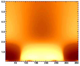
Figure 3: (a): Scheme for the computation of the potential energy of two tripoles ${\sf C}^{3}_{\rm I}$ and ${\sf C}^{3}_{\rm J}$ that form a charged doublet d; and (b): the potential energy of d corresponding to $\phi,\theta,\chi,\xi=0$ and $\rho_{\rm I}=\rho_{\rm J}=\rho_{\circ}/\sqrt{3}$. The position angle ($\zeta$) of ${\sf C}^{3}_{\rm J}$ with respect to ${\sf C}^{3}_{\rm I}$ is shown along the horizontal axis (in degrees); the vertical axis is the distance between two particles (in units of $\rho_{\circ}$). The darker regions correspond to lower energies.

4 Two-component systems of tripoles

A part of the field of the tripole (in its equatorial plane) is ring-closed [24], whereas another part is extended (over the ring’s poles). In its equatorial plane, the tripole possesses $2\pi\frac{m}{n}$-rotational symmetry ($m\leq n-1$, $n=2,3$) of the second- and third-order cyclic groups. With the dispersion of colour-charges, corresponding to this symmetry, different $\triangle$-tripoles can combine into chains.

A pair of tripoles would combine pole-to-pole with each other forming a doublet (d). One can estimate the potential energy of this system by computing the pair-wise forces between its constituents. The scheme for this computation is shown in Fig.3(a). The potential energy of the doublet depends on the positions of its components with respect to each other. It can be computed as a superposition ($V_{\Sigma}$) of two potentials, $V_{\ominus}=-\int{F_{\ominus}}$ and $V_{\oplus}=-\int{F_{\oplus}}$, based on the split field (9). That is,

$$\begin{split}&V_{\ominus}(\rho_{ij})=s_{ij}\rho_{ij}\exp{(-\rho_{ij}^{-1})}+\operatorname{Ei}{(-\rho_{ij}^{-1})},\\ &V_{\oplus}(\rho_{ij})=-s_{ij}\exp{(-\rho_{ij}^{-1})},\end{split}$$ (25)

where $\rho_{ij}$ is the distance between the $i$-th charge of the tripole  ${\begin{turn}{-180.0}\raisebox{-7.19025pt}{\begin{turn}{-180.0}\raisebox{-7.19025pt}{\sf C}\end{turn}}\end{turn}}\raisebox{4.73611pt}{\tiny\begin{turn}{-180.0}\raisebox{-3.59512pt}{\begin{turn}{-180.0}\raisebox{-3.59512pt}{$+$}\end{turn}}\end{turn} \hskip 2.15277pt{\scriptsize\begin{turn}{-180.0}\raisebox{-5.03317pt}{\begin{turn}{-180.0}\raisebox{-5.03317pt}{$3$}\end{turn}}\end{turn}}}_{\rm I}$ and $j$-th charge of the tripole  ${\begin{turn}{-180.0}\raisebox{-7.19025pt}{\begin{turn}{-180.0}\raisebox{-7.19025pt}{\sf C}\end{turn}}\end{turn}}\raisebox{4.73611pt}{\tiny\begin{turn}{-180.0}\raisebox{-3.59512pt}{\begin{turn}{-180.0}\raisebox{-3.59512pt}{$+$}\end{turn}}\end{turn} \hskip 2.15277pt{\scriptsize\begin{turn}{-180.0}\raisebox{-5.03317pt}{\begin{turn}{-180.0}\raisebox{-5.03317pt}{$3$}\end{turn}}\end{turn}}}_{\rm J}$; $i,j\in\{1,2,3\}$. For the sake of simplicity the arbitrary constants of integration in (25) are set to zero. If we assume (also for simplicity) that the relative positions of the primitive charges constituting the two tripoles of the doublet are fixed within each of these tripoles, then $V_{\Sigma}$ will have nine terms corresponding to the positions of the three charges of one tripole with respect to the three charges of the other:

$$V_{\Sigma}=-\mathbf{w}^{\intercal}V\mathbf{w}.$$ (26)

Here the elements ${\rm v}_{ij}$ of the $3\times 3$ matrix $V$ are the following:

$${\rm v}_{ij}=[V_{\ominus}(\rho_{ij})+V_{\oplus}(\rho_{ij})]\hat{c}_{ik}\hat{c}^{kj},$$ (27)

$$\hat{c}_{ik}=c_{ik}+\delta_{ik},\hskip 14.22636pt\hat{c}_{kj}=c_{kj}+\delta_{kj}$$ (28)

(repeated indices are summed over), where $c_{ik}$, $c_{kj}$ are the matrix elements of, respectively,  ${\begin{turn}{-180.0}\raisebox{-7.19025pt}{\begin{turn}{-180.0}\raisebox{-7.19025pt}{\sf C}\end{turn}}\end{turn}}\raisebox{4.73611pt}{\tiny\begin{turn}{-180.0}\raisebox{-3.59512pt}{\begin{turn}{-180.0}\raisebox{-3.59512pt}{$+$}\end{turn}}\end{turn} \hskip 2.15277pt{\scriptsize\begin{turn}{-180.0}\raisebox{-5.03317pt}{\begin{turn}{-180.0}\raisebox{-5.03317pt}{$3$}\end{turn}}\end{turn}}}_{\rm I}$ and  ${\begin{turn}{-180.0}\raisebox{-7.19025pt}{\begin{turn}{-180.0}\raisebox{-7.19025pt}{\sf C}\end{turn}}\end{turn}}\raisebox{4.73611pt}{\tiny\begin{turn}{-180.0}\raisebox{-3.59512pt}{\begin{turn}{-180.0}\raisebox{-3.59512pt}{$+$}\end{turn}}\end{turn} \hskip 2.15277pt{\scriptsize\begin{turn}{-180.0}\raisebox{-5.03317pt}{\begin{turn}{-180.0}\raisebox{-5.03317pt}{$3$}\end{turn}}\end{turn}}}_{\rm J}$; the distances $\rho_{ij}$ are those between the charges $i$ and $j$ belonging, respectively, to the tripoles  ${\begin{turn}{-180.0}\raisebox{-7.19025pt}{\begin{turn}{-180.0}\raisebox{-7.19025pt}{\sf C}\end{turn}}\end{turn}}\raisebox{4.73611pt}{\tiny\begin{turn}{-180.0}\raisebox{-3.59512pt}{\begin{turn}{-180.0}\raisebox{-3.59512pt}{$+$}\end{turn}}\end{turn} \hskip 2.15277pt{\scriptsize\begin{turn}{-180.0}\raisebox{-5.03317pt}{\begin{turn}{-180.0}\raisebox{-5.03317pt}{$3$}\end{turn}}\end{turn}}}_{\rm I}$ and  ${\begin{turn}{-180.0}\raisebox{-7.19025pt}{\begin{turn}{-180.0}\raisebox{-7.19025pt}{\sf C}\end{turn}}\end{turn}}\raisebox{4.73611pt}{\tiny\begin{turn}{-180.0}\raisebox{-3.59512pt}{\begin{turn}{-180.0}\raisebox{-3.59512pt}{$+$}\end{turn}}\end{turn} \hskip 2.15277pt{\scriptsize\begin{turn}{-180.0}\raisebox{-5.03317pt}{\begin{turn}{-180.0}\raisebox{-5.03317pt}{$3$}\end{turn}}\end{turn}}}_{\rm J}$; and the indices $i,j,k=1,2,3$ correspond to the three primary colours. The signature $s_{ij}$ in (25) is computed with the use of (15). The Kronecker delta-symbols in (28) are added to the elements $c_{ik}$ and $c_{kj}$ to satisfy the boundary condition of mutual cancellation (colourlessness) of three complementary colour charges at infinity.

Besides its translational ($\mathbf{\rho}_{\rm IJ}$) and rotational ($\chi,\xi,\zeta$) degrees of freedom, the doublet d has two degrees of freedom corresponding to the radial oscillations of its components (radii $\rho_{\rm I}$ and $\rho_{\rm J}$). Making use of some obvious symmetries, we can reduce the dimensionality of the case (without loosing much information) by putting $\phi,\theta,\chi,\xi=0$ and setting $\rho_{\rm I}$ and $\rho_{\rm J}$ to some fixed values, say, to the tripole’s equilibrium radius ($\rho_{\circ}/\sqrt{3}$). The potential energy of this configuration is mapped in Fig.3(b) as a function of $\rho_{\rm IJ}$ and $\zeta$. It is seen that two like-charged tripoles can attract each other, if $\zeta\approx\pi$ and $\rho_{\rm IJ}>2\rho_{\circ}$. The sign of the force between the tripoles depends on the position angle: for the angle $\zeta=\pi/2$ the force is vanishing; it is attractive for $\pi/2<\zeta\leq 3\pi/2$:

$$\begin{split}{{\begin{turn}{-180.0}\raisebox{-7.19025pt}{\begin{turn}{-180.0}\raisebox{-7.19025pt}{$\triangle$}\end{turn}}\end{turn}}\raisebox{0.86108pt}{\tiny\begin{turn}{-180.0}\raisebox{-3.59512pt}{\begin{turn}{-180.0}\raisebox{-3.59512pt}{$+$}\end{turn}}\end{turn}}\raisebox{4.30554pt}{\tiny\begin{turn}{-180.0}\raisebox{-3.59512pt}{\begin{turn}{-180.0}\raisebox{-3.59512pt}{$\blacktriangle$}\end{turn}}\end{turn}}\hskip 2.15277pt}\rightarrow&\leftarrow\begin{turn}{-180.0}\raisebox{-7.19025pt}{ {\begin{turn}{-180.0}\raisebox{-7.19025pt}{\begin{turn}{-180.0}\raisebox{-7.19025pt}{$\triangle$}\end{turn}}\end{turn}}\raisebox{0.86108pt}{\tiny\begin{turn}{-180.0}\raisebox{-3.59512pt}{\begin{turn}{-180.0}\raisebox{-3.59512pt}{$+$}\end{turn}}\end{turn}}\raisebox{4.30554pt}{\tiny\begin{turn}{-180.0}\raisebox{-3.59512pt}{\begin{turn}{-180.0}\raisebox{-3.59512pt}{$\blacktriangle$}\end{turn}}\end{turn}}\hskip 2.15277pt}\end{turn}\\ {{\begin{turn}{-180.0}\raisebox{-7.19025pt}{\begin{turn}{-180.0}\raisebox{-7.19025pt}{$\triangle$}\end{turn}}\end{turn}}\raisebox{0.86108pt}{\tiny\begin{turn}{-180.0}\raisebox{-3.59512pt}{\begin{turn}{-180.0}\raisebox{-3.59512pt}{$+$}\end{turn}}\end{turn}}\raisebox{4.30554pt}{\tiny\begin{turn}{-180.0}\raisebox{-3.59512pt}{\begin{turn}{-180.0}\raisebox{-3.59512pt}{$\blacktriangle$}\end{turn}}\end{turn}}\hskip 2.15277pt}\rightarrow&\leftarrow~{}{{\begin{turn}{-180.0}\raisebox{-7.19025pt}{\begin{turn}{-180.0}\raisebox{-7.19025pt}{$\triangle$}\end{turn}}\end{turn}}\raisebox{1.07639pt}{\tiny\begin{turn}{-180.0}\raisebox{-3.59512pt}{\begin{turn}{-180.0}\raisebox{-3.59512pt}{$+$}\end{turn}}\end{turn}}\raisebox{0.43057pt}{\tiny\begin{turn}{-180.0}\raisebox{-3.59512pt}{\begin{turn}{-180.0}\raisebox{-3.59512pt}{$\blacktriangle$}\end{turn}}\end{turn}}\hskip 0.43057pt}\\ {{\begin{turn}{-180.0}\raisebox{-7.19025pt}{\begin{turn}{-180.0}\raisebox{-7.19025pt}{$\triangle$}\end{turn}}\end{turn}}\raisebox{0.86108pt}{\tiny\begin{turn}{-180.0}\raisebox{-3.59512pt}{\begin{turn}{-180.0}\raisebox{-3.59512pt}{$+$}\end{turn}}\end{turn}}\raisebox{4.30554pt}{\tiny\begin{turn}{-180.0}\raisebox{-3.59512pt}{\begin{turn}{-180.0}\raisebox{-3.59512pt}{$\blacktriangle$}\end{turn}}\end{turn}}\hskip 2.15277pt}\rightarrow&\leftarrow~{}{{\begin{turn}{-180.0}\raisebox{-7.19025pt}{\begin{turn}{-180.0}\raisebox{-7.19025pt}{$\triangle$}\end{turn}}\end{turn}}\raisebox{1.29167pt}{\tiny\begin{turn}{-180.0}\raisebox{-3.59512pt}{\begin{turn}{-180.0}\raisebox{-3.59512pt}{$+$}\end{turn}}\end{turn}}\raisebox{0.43057pt}{\tiny\begin{turn}{-180.0}\raisebox{-3.59512pt}{\begin{turn}{-180.0}\raisebox{-3.59512pt}{$\blacktriangle$}\end{turn}}\end{turn}}\hskip 0.86108pt}~{}\end{split}$$ (29)

and repulsive for $\lvert\zeta\rvert<\pi/2$:

$$\begin{split}\leftarrow~{}{{\begin{turn}{-180.0}\raisebox{-7.19025pt}{\begin{turn}{-180.0}\raisebox{-7.19025pt}{$\triangle$}\end{turn}}\end{turn}}\raisebox{0.86108pt}{\tiny\begin{turn}{-180.0}\raisebox{-3.59512pt}{\begin{turn}{-180.0}\raisebox{-3.59512pt}{$+$}\end{turn}}\end{turn}}\raisebox{4.30554pt}{\tiny\begin{turn}{-180.0}\raisebox{-3.59512pt}{\begin{turn}{-180.0}\raisebox{-3.59512pt}{$\blacktriangle$}\end{turn}}\end{turn}}\hskip 2.15277pt}\hskip 17.07182pt&\hskip 17.07182pt{{\begin{turn}{-180.0}\raisebox{-7.19025pt}{\begin{turn}{-180.0}\raisebox{-7.19025pt}{$\triangle$}\end{turn}}\end{turn}}\raisebox{0.86108pt}{\tiny\begin{turn}{-180.0}\raisebox{-3.59512pt}{\begin{turn}{-180.0}\raisebox{-3.59512pt}{$+$}\end{turn}}\end{turn}}\raisebox{4.30554pt}{\tiny\begin{turn}{-180.0}\raisebox{-3.59512pt}{\begin{turn}{-180.0}\raisebox{-3.59512pt}{$\blacktriangle$}\end{turn}}\end{turn}}\hskip 2.15277pt}\rightarrow~{}\\ \leftarrow~{}{{\begin{turn}{-180.0}\raisebox{-7.19025pt}{\begin{turn}{-180.0}\raisebox{-7.19025pt}{$\triangle$}\end{turn}}\end{turn}}\raisebox{0.86108pt}{\tiny\begin{turn}{-180.0}\raisebox{-3.59512pt}{\begin{turn}{-180.0}\raisebox{-3.59512pt}{$+$}\end{turn}}\end{turn}}\raisebox{4.30554pt}{\tiny\begin{turn}{-180.0}\raisebox{-3.59512pt}{\begin{turn}{-180.0}\raisebox{-3.59512pt}{$\blacktriangle$}\end{turn}}\end{turn}}\hskip 2.15277pt}\hskip 17.07182pt&\hskip 14.22636pt\begin{turn}{-180.0}\raisebox{-7.19025pt}{ {\begin{turn}{-180.0}\raisebox{-7.19025pt}{\begin{turn}{-180.0}\raisebox{-7.19025pt}{$\triangle$}\end{turn}}\end{turn}}\raisebox{1.07639pt}{\tiny\begin{turn}{-180.0}\raisebox{-3.59512pt}{\begin{turn}{-180.0}\raisebox{-3.59512pt}{$+$}\end{turn}}\end{turn}}\raisebox{0.43057pt}{\tiny\begin{turn}{-180.0}\raisebox{-3.59512pt}{\begin{turn}{-180.0}\raisebox{-3.59512pt}{$\blacktriangle$}\end{turn}}\end{turn}}\hskip 0.43057pt}\end{turn}\rightarrow\\ \leftarrow~{}{{\begin{turn}{-180.0}\raisebox{-7.19025pt}{\begin{turn}{-180.0}\raisebox{-7.19025pt}{$\triangle$}\end{turn}}\end{turn}}\raisebox{0.86108pt}{\tiny\begin{turn}{-180.0}\raisebox{-3.59512pt}{\begin{turn}{-180.0}\raisebox{-3.59512pt}{$+$}\end{turn}}\end{turn}}\raisebox{4.30554pt}{\tiny\begin{turn}{-180.0}\raisebox{-3.59512pt}{\begin{turn}{-180.0}\raisebox{-3.59512pt}{$\blacktriangle$}\end{turn}}\end{turn}}\hskip 2.15277pt}\hskip 17.07182pt&\hskip 14.22636pt\begin{turn}{-180.0}\raisebox{-7.19025pt}{ {\begin{turn}{-180.0}\raisebox{-7.19025pt}{\begin{turn}{-180.0}\raisebox{-7.19025pt}{$\triangle$}\end{turn}}\end{turn}}\raisebox{1.29167pt}{\tiny\begin{turn}{-180.0}\raisebox{-3.59512pt}{\begin{turn}{-180.0}\raisebox{-3.59512pt}{$+$}\end{turn}}\end{turn}}\raisebox{0.43057pt}{\tiny\begin{turn}{-180.0}\raisebox{-3.59512pt}{\begin{turn}{-180.0}\raisebox{-3.59512pt}{$\blacktriangle$}\end{turn}}\end{turn}} \hskip 0.86108pt}\end{turn}\rightarrow~{}.\end{split}$$ (30)

Thus, separated by distance $\rho_{\rm IJ}>2\rho_{\circ}$ two tripoles can combine into the configuration

$${\sf d}^{+}={{\begin{turn}{-180.0}\raisebox{-7.19025pt}{\begin{turn}{-180.0}\raisebox{-7.19025pt}{$\triangle$}\end{turn}}\end{turn}}\raisebox{0.86108pt}{\tiny\begin{turn}{-180.0}\raisebox{-3.59512pt}{\begin{turn}{-180.0}\raisebox{-3.59512pt}{$+$}\end{turn}}\end{turn}}\raisebox{4.30554pt}{\tiny\begin{turn}{-180.0}\raisebox{-3.59512pt}{\begin{turn}{-180.0}\raisebox{-3.59512pt}{$\blacktriangle$}\end{turn}}\end{turn}}\hskip 2.15277pt}\begin{turn}{-180.0}\raisebox{-7.19025pt}{ {\begin{turn}{-180.0}\raisebox{-7.19025pt}{\begin{turn}{-180.0}\raisebox{-7.19025pt}{$\triangle$}\end{turn}}\end{turn}}\raisebox{0.86108pt}{\tiny\begin{turn}{-180.0}\raisebox{-3.59512pt}{\begin{turn}{-180.0}\raisebox{-3.59512pt}{$+$}\end{turn}}\end{turn}}\raisebox{4.30554pt}{\tiny\begin{turn}{-180.0}\raisebox{-3.59512pt}{\begin{turn}{-180.0}\raisebox{-3.59512pt}{$\blacktriangle$}\end{turn}}\end{turn}}\hskip 2.15277pt}\end{turn}\hskip 14.22636pt(\text{or}\hskip 14.22636pt{\sf d}^{-}={\begin{turn}{-180.0}\raisebox{-7.19025pt}{\begin{turn}{-180.0}\raisebox{-7.19025pt}{$\triangle$}\end{turn}}\end{turn}}\raisebox{0.86108pt}{\tiny\begin{turn}{-180.0}\raisebox{-3.59512pt}{\begin{turn}{-180.0}\raisebox{-3.59512pt}{$-$}\end{turn}}\end{turn}}\raisebox{4.30554pt}{\tiny\begin{turn}{-180.0}\raisebox{-3.59512pt}{\begin{turn}{-180.0}\raisebox{-3.59512pt}{$\blacktriangle$}\end{turn}}\end{turn}}\hskip 2.15277pt\begin{turn}{-180.0}\raisebox{-7.19025pt}{ {\begin{turn}{-180.0}\raisebox{-7.19025pt}{\begin{turn}{-180.0}\raisebox{-7.19025pt}{$\triangle$}\end{turn}}\end{turn}}\raisebox{0.86108pt}{\tiny\begin{turn}{-180.0}\raisebox{-3.59512pt}{\begin{turn}{-180.0}\raisebox{-3.59512pt}{$-$}\end{turn}}\end{turn}}\raisebox{4.30554pt}{\tiny\begin{turn}{-180.0}\raisebox{-3.59512pt}{\begin{turn}{-180.0}\raisebox{-3.59512pt}{$\blacktriangle$}\end{turn}}\end{turn}}\hskip 2.15277pt}\end{turn}~{}).$$ (31)

The existence of bifurcation points in the potential at $\rho_{\rm IJ}\approx 2\rho_{\circ}$ suggests the possibility of moving the system into a deeper potential well at $\rho\approx 0$ by squeezing it below $\rho_{\rm IJ}=\rho_{\circ}$ (and keeping $\zeta=0$).

The width of the central potential well ($\zeta=\pi$, $\rho_{\rm IJ}>2\rho_{\circ}$) allows a certain degree of freedom for the constituents of d to oscillate (rotating) within $\frac{2}{3}\pi<\zeta<\frac{4}{3}\pi$:

$${\sf d}^{+}_{\upharpoonright}={{\begin{turn}{-180.0}\raisebox{-7.19025pt}{\begin{turn}{-180.0}\raisebox{-7.19025pt}{$\triangle$}\end{turn}}\end{turn}}\raisebox{0.86108pt}{\tiny\begin{turn}{-180.0}\raisebox{-3.59512pt}{\begin{turn}{-180.0}\raisebox{-3.59512pt}{$+$}\end{turn}}\end{turn}}\raisebox{4.30554pt}{\tiny\begin{turn}{-180.0}\raisebox{-3.59512pt}{\begin{turn}{-180.0}\raisebox{-3.59512pt}{$\blacktriangle$}\end{turn}}\end{turn}}\hskip 2.15277pt}\hskip 3.87495pt{{\begin{turn}{-180.0}\raisebox{-7.19025pt}{\begin{turn}{-180.0}\raisebox{-7.19025pt}{$\triangle$}\end{turn}}\end{turn}}\raisebox{1.07639pt}{\tiny\begin{turn}{-180.0}\raisebox{-3.59512pt}{\begin{turn}{-180.0}\raisebox{-3.59512pt}{$+$}\end{turn}}\end{turn}}\raisebox{0.43057pt}{\tiny\begin{turn}{-180.0}\raisebox{-3.59512pt}{\begin{turn}{-180.0}\raisebox{-3.59512pt}{$\blacktriangle$}\end{turn}}\end{turn}}\hskip 0.43057pt}\hskip 5.69046pt\rightleftarrows\hskip 5.69046pt{\sf d}^{+}_{\downharpoonright}={\begin{turn}{-180.0}\raisebox{-7.19025pt}{\begin{turn}{-180.0}\raisebox{-7.19025pt}{$\triangle$}\end{turn}}\end{turn}}\raisebox{0.86108pt}{\tiny\begin{turn}{-180.0}\raisebox{-3.59512pt}{\begin{turn}{-180.0}\raisebox{-3.59512pt}{$+$}\end{turn}}\end{turn}}\raisebox{4.30554pt}{\tiny\begin{turn}{-180.0}\raisebox{-3.59512pt}{\begin{turn}{-180.0}\raisebox{-3.59512pt}{$\blacktriangle$}\end{turn}}\end{turn}}\hskip 2.15277pt\hskip 3.87495pt{{\begin{turn}{-180.0}\raisebox{-7.19025pt}{\begin{turn}{-180.0}\raisebox{-7.19025pt}{$\triangle$}\end{turn}}\end{turn}}\raisebox{1.29167pt}{\tiny\begin{turn}{-180.0}\raisebox{-3.59512pt}{\begin{turn}{-180.0}\raisebox{-3.59512pt}{$+$}\end{turn}}\end{turn}}\raisebox{0.43057pt}{\tiny\begin{turn}{-180.0}\raisebox{-3.59512pt}{\begin{turn}{-180.0}\raisebox{-3.59512pt}{$\blacktriangle$}\end{turn}}\end{turn}}\hskip 0.86108pt}~{}.$$ (32)

The strength and sign of the force between the components depends on $\zeta$. This implies the distance $\rho_{\rm IJ}$ being covariant with $\zeta$; that is, the translational and rotational oscillations of the doublet are synchronous. Note that in (31) and (32) we put the symbols  $\triangle$ $+$    side-by-side, implying, however, that they rotate coaxially with respect to each other ($\theta,\xi=0$). The symbols $\upharpoonright$ and $\downharpoonright$ in (32) denote the clockwise and anticlockwise rotations. Over again, we would like to stress that the diagrams (29)-(32) express not otherwise than structural relationships (like, for instance, the formulae in organic chemistry), and by no means should they be mistaken for algebraic expressions.

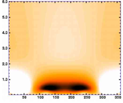
Figure 4: Potential of the tripole-antitripole system ${\sf d}^{\circ}$

Similarly to the structure of the charged doublet, a pair of oppositely charged tripoles can form a neutral doublet

$${\sf d}^{\circ}={\begin{turn}{-180.0}\raisebox{-7.19025pt}{\begin{turn}{-180.0}\raisebox{-7.19025pt}{$\triangle$}\end{turn}}\end{turn}}\raisebox{0.86108pt}{\tiny\begin{turn}{-180.0}\raisebox{-3.59512pt}{\begin{turn}{-180.0}\raisebox{-3.59512pt}{$-$}\end{turn}}\end{turn}}\raisebox{4.30554pt}{\tiny\begin{turn}{-180.0}\raisebox{-3.59512pt}{\begin{turn}{-180.0}\raisebox{-3.59512pt}{$\blacktriangle$}\end{turn}}\end{turn}}\hskip 2.15277pt\begin{turn}{-180.0}\raisebox{-7.19025pt}{ {\begin{turn}{-180.0}\raisebox{-7.19025pt}{\begin{turn}{-180.0}\raisebox{-7.19025pt}{$\triangle$}\end{turn}}\end{turn}}\raisebox{0.86108pt}{\tiny\begin{turn}{-180.0}\raisebox{-3.59512pt}{\begin{turn}{-180.0}\raisebox{-3.59512pt}{$+$}\end{turn}}\end{turn}}\raisebox{4.30554pt}{\tiny\begin{turn}{-180.0}\raisebox{-3.59512pt}{\begin{turn}{-180.0}\raisebox{-3.59512pt}{$\blacktriangle$}\end{turn}}\end{turn}}\hskip 2.15277pt}\end{turn}~{}.$$ (33)

The corresponding potential is shown in Fig.4. This system is massless, as well as colour-neutral (with $q_{{\sf d}^{\circ}}=0$, $m_{{\sf d}^{\circ}}=0$, and $\tilde{m}_{{\sf d}^{\circ}}=0$). Like ${\sf d}^{+}$ and ${\sf d}^{-}$, the neutral doublet would oscillate, albeit with a smaller amplitude of its translational mode of oscillations because its constituents are confined within a deep potential well at $\rho_{\rm IJ}\sim 0.5\rho_{\circ}$, as seen in Fig.4. The rotational degree of freedom of the tripoles constituting the neutral doublet corresponds to $\zeta=\pi\pm\pi/3$.

The dynamics of the charged and neutral doublets deserves a more detailed study but we shall address this problem elsewhere, since here we are interested mostly in reviewing the variety of possible particle configurations.

5 Three-component strings of tripoles

A three-component string of $\triangle$-shaped tripoles [see Fig.5(a)] have at least fifteen degrees of freedom (not taking into account possible flexions of the string). Making use of obvious symmetries we can reduce the number of parameters and analyse a basic case of an open string with three equidistant coaxial tripoles, $\triangle_{\rm I}$, $\triangle_{\rm J}$ and $\triangle_{\rm K}$. The potential of this system for the case $\rho_{\rm IJ}=\rho_{\rm JK}=\rho$ and $\zeta_{\rm K}=2\zeta_{\rm J}$ is shown in Fig.5(b).

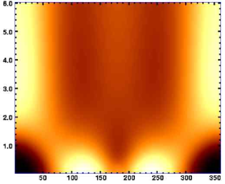
Figure 5: (a): An open-string configuration of three coaxial tripoles $\triangle_{\rm I}$, $\triangle_{\rm J}$, $\triangle_{\rm K}$, and (b): its potential for the case $\rho_{\rm IJ}=\rho_{\rm JK}=\rho$, $\zeta_{\rm K}=2\zeta_{\rm J}$.

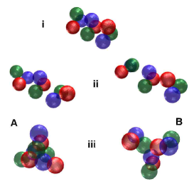
Figure 6: (a): Open string (i) formed of three $\triangle$-tripoles is flexible: the loose ends of the string attract each other causing its closure in a loop. Two different bending directions (ii) correspond to two possible configurations of the loop (iii), one with the vertices of its constituents directed outwards from the loop (A) and another – inwards (B). (b): The scheme of the closed string.

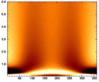
Figure 7: Potential of the three-component closed string ${\tt Y}$ as a function: (a) of the position angle $\zeta$ between the $\triangle$-constituents of the string; and (b) of their phase angle $\phi$ for the fixed $\zeta=120^{\circ}$. The vertical axes in both plots correspond to radius $\rho_{\tt Y}$ (in units of $\rho_{\circ}$).

For $\rho>2\rho_{\circ}$ there are two potential wells corresponding to the position angle $\zeta=\pm\frac{2}{3}\pi$. Similarly to the doublet d, the three-component string would perform translational and rotational oscillations which, however, cannot be stable because of various bifurcation points in its potential (Fig.5(b)). At the same time, one can see that the tripoles at the ends of the string attract each other, like those shown in the diagram (29), and, due to the possible flexional deformations, the string $\triangle$ $\blacktriangle$   $\triangle$ $\blacktriangle$   $\triangle$ $\blacktriangle$   will necessarily close into a symmetric loop

$${\tt Y}:=\raisebox{-6.02773pt}{\begin{turn}{-180.0}\raisebox{-7.19025pt}{ {\begin{turn}{-180.0}\raisebox{-7.19025pt}{\begin{turn}{-180.0}\raisebox{-7.19025pt}{$\triangle$}\end{turn}}\end{turn}}\raisebox{4.30554pt}{\tiny\begin{turn}{-180.0}\raisebox{-3.59512pt}{\begin{turn}{-180.0}\raisebox{-3.59512pt}{$\blacktriangle$}\end{turn}}\end{turn}}\hskip 2.15277pt}\end{turn}}\raisebox{6.45831pt}{\begin{turn}{-180.0}\raisebox{-7.19025pt}{ {\begin{turn}{-180.0}\raisebox{-7.19025pt}{\begin{turn}{-180.0}\raisebox{-7.19025pt}{$\triangle$}\end{turn}}\end{turn}}\raisebox{0.43057pt}{\tiny\begin{turn}{-180.0}\raisebox{-3.59512pt}{\begin{turn}{-180.0}\raisebox{-3.59512pt}{$\blacktriangle$}\end{turn}}\end{turn}} \hskip 0.86108pt}\end{turn}}\raisebox{-6.45831pt}{\begin{turn}{-180.0}\raisebox{-7.19025pt}{ {\begin{turn}{-180.0}\raisebox{-7.19025pt}{\begin{turn}{-180.0}\raisebox{-7.19025pt}{$\triangle$}\end{turn}}\end{turn}}\raisebox{0.43057pt}{\tiny\begin{turn}{-180.0}\raisebox{-3.59512pt}{\begin{turn}{-180.0}\raisebox{-3.59512pt}{$\blacktriangle$}\end{turn}}\end{turn}}\hskip 0.43057pt}\end{turn}}$$ (34)

as shown in Fig.6. This closure changes the properties of the system: in the case of the open string the variation of its phase angle $\phi$ [see Fig.5(a)] will not change the binding energy (relative distances) between its constituents, whereas the energy of the ring-closed configuration, Fig.6(b), is phase-dependent. Obviously, the energy states of the configurations A ($\phi=\pi$) and B ($\phi=0$) in Fig.6(a) are distinct. In fact, these two configurations can be seen as $\pi$-phase-shifted states of the same structure, in which its constituents, the $\triangle$-shaped tripoles, spin around its ring-axis. As in the case of the two-component system, the rotation of tripoles around the ring-axis of ${\tt Y}$ implies their circular translation along this axis, as well as the radial oscillations of ${\tt Y}$. This can be seen by analysing Fig.7, where the potential energy of ${\tt Y}$ is mapped as a function of the radius, $\rho_{\tt Y}$, position angle $\zeta$, and phase angle $\phi$ between the components of the system.

The potential wells in Fig.7(a) correspond to the position angles $\zeta\approx\pm\frac{2}{3}\pi$ for a wide range of $\rho_{\tt Y}$. The charges spinning around the ring-closed axis of ${\tt Y}$ (clockwise or anticlockwise) will generate a toroidal (ring-closed) magnetic field which, at the same time, will force these charges to move along the torus. This circular motion of charges will generate a secondary (poloidal) magnetic field, contributing to the spin of these charges around the ring-axis, and so forth. The strength of the magnetic field will be covariant with respect to $\rho_{\tt Y}$. The interplay of the varying toroidal and poloidal magnetic fields, oscillating $\rho_{\tt Y}$, and varying velocities of the rotating charges converts this system into a complicated harmonic oscillator with a series of eigenfrequences and oscillatory modes.

The trajectories of charges (electric currents) in ${\tt Y}$, which are shown in Fig.8,

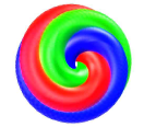
Figure 8: Trajectories of the colour charges (electric currents) in the structure ${\tt Y}$. The charges spin about the ring-axis of this structure and, at the same time, synchroneously translate along this axis.

are helices with constant pitch and with two possible helical signs: ${\tt Y}_{\upharpoonright}$ (clockwise) or ${\tt Y}_{\downharpoonright}$ (anticlockwise), corresponding to two different signs of the internal angular momentum of the constituents of this structure (around the ring-closed axis). Due to synchronisation of frequencies [25], by the closure of each $2\pi$-path along the ring-axis of ${\tt Y}$ the currents are additionally $\pi$-twisted about this axis. They need to travel twice along the ring to meet their initial phase condition (A or B). The system looks much like a toroidal solenoid coil with winding number $w_{\tt Y}=3$.

It is plain to see that if ${\tt Y}$ is positively charged, the vectors of its angular momentum and magnetic moment are always parallel (pointing in the same direction)

$$\overset{\stackrel{{\scriptstyle{\tiny\ell}\rightarrow}}{{\raisebox{0.43057pt}{\tiny{\sf B}$\rightarrow$}}}}{{\tt Y}^{+}}$$

whereas in the case of the negatively charged ${\tt Y}$ these vectors are antiparallel:

$$\overset{\stackrel{{\scriptstyle{\tiny\ell}\rightarrow}}{{\raisebox{0.43057pt}{\tiny$\leftarrow$ {\sf B}}}}}{{\tt Y}^{-}}.$$

This property must be taken into account when considering interactions between different Y-particles. The charge and mass of ${\tt Y}$ roughly correspond to the sum of the charges and masses of its nine constituents: $q_{\tt Y}=\pm 9$ (in units of $q_{\circ}$), $m_{\tt Y}=\tilde{m}_{\tt Y}=9$ (in units of $m_{\circ}$). At large distances from ${\tt Y}$ the combined chromofield of its constituents is colour-neutral and almost spherically symmetric. Thus, separated by large distances, ${\tt Y}$-particles would behave as point-like colourless charges. At small distances from the particle one must take into account the chromatic polarisation of the field.

6 Chains of unlike-charged tripoles

Hereafter – in order to simplify our analysis – we shall use the observation that $\triangle$-shaped tripoles, when clustered, form alike structures on different levels of complexity. For instance, a simple $\triangle$-tripole and the more complicated ring-closed triplet Y (which consists of three $\triangle$-tripoles), both possess the same $\frac{2}{3}\pi$-rotational symmetry. Then (up to a certain limit) one can use the same combinatoric rules when dealing with structures based on Y- and $\triangle$-particles. However, some new properties emerging on higher levels of complexity must be taken into account, such as, for example, the helicity property of Y, which by no means can be found in $\triangle$. Based on the resemblance between different complexity levels, and using the pattern of attraction and repulsion between the tripoles with different positional angles [shown in the diagrams (29) and (30)] , let us explore the variety of possible structures based on the tripolar charges. Of course, the detailed study of these structures and their properties need more rigorous numerical calculations and simulations, which we shall discuss elsewhere.

Based on the pattern (29) - (30), one can find that the unlike-charged doublets, ${\sf d}^{-}$ and ${\sf d}^{+}$, can combine and form chains with two possible rotations of the components with respect to each other, clockwise:

$${\sf d}^{\circ}_{2\upharpoonright}={\begin{turn}{-180.0}\raisebox{-7.19025pt}{\begin{turn}{-180.0}\raisebox{-7.19025pt}{$\triangle$}\end{turn}}\end{turn}}\raisebox{0.86108pt}{\tiny\begin{turn}{-180.0}\raisebox{-3.59512pt}{\begin{turn}{-180.0}\raisebox{-3.59512pt}{$-$}\end{turn}}\end{turn}}\raisebox{4.30554pt}{\tiny\begin{turn}{-180.0}\raisebox{-3.59512pt}{\begin{turn}{-180.0}\raisebox{-3.59512pt}{$\blacktriangle$}\end{turn}}\end{turn}}\hskip 2.15277pt~{}{{\begin{turn}{-180.0}\raisebox{-7.19025pt}{\begin{turn}{-180.0}\raisebox{-7.19025pt}{$\triangle$}\end{turn}}\end{turn}}\raisebox{1.07639pt}{\tiny\begin{turn}{-180.0}\raisebox{-3.59512pt}{\begin{turn}{-180.0}\raisebox{-3.59512pt}{$-$}\end{turn}}\end{turn}}\raisebox{0.43057pt}{\tiny\begin{turn}{-180.0}\raisebox{-3.59512pt}{\begin{turn}{-180.0}\raisebox{-3.59512pt}{$\blacktriangle$}\end{turn}}\end{turn}}\hskip 0.43057pt}\begin{turn}{-180.0}\raisebox{-7.19025pt}{ {\begin{turn}{-180.0}\raisebox{-7.19025pt}{\begin{turn}{-180.0}\raisebox{-7.19025pt}{$\triangle$}\end{turn}}\end{turn}}\raisebox{1.07639pt}{\tiny\begin{turn}{-180.0}\raisebox{-3.59512pt}{\begin{turn}{-180.0}\raisebox{-3.59512pt}{$+$}\end{turn}}\end{turn}}\raisebox{0.43057pt}{\tiny\begin{turn}{-180.0}\raisebox{-3.59512pt}{\begin{turn}{-180.0}\raisebox{-3.59512pt}{$\blacktriangle$}\end{turn}}\end{turn}}\hskip 0.43057pt}\end{turn}\begin{turn}{-180.0}\raisebox{-7.19025pt}{ {\begin{turn}{-180.0}\raisebox{-7.19025pt}{\begin{turn}{-180.0}\raisebox{-7.19025pt}{$\triangle$}\end{turn}}\end{turn}}\raisebox{0.86108pt}{\tiny\begin{turn}{-180.0}\raisebox{-3.59512pt}{\begin{turn}{-180.0}\raisebox{-3.59512pt}{$+$}\end{turn}}\end{turn}}\raisebox{4.30554pt}{\tiny\begin{turn}{-180.0}\raisebox{-3.59512pt}{\begin{turn}{-180.0}\raisebox{-3.59512pt}{$\blacktriangle$}\end{turn}}\end{turn}}\hskip 2.15277pt}\end{turn}$$ (35)

or anticlockwise:

$${\sf d}^{\circ}_{2\downharpoonright}={\begin{turn}{-180.0}\raisebox{-7.19025pt}{\begin{turn}{-180.0}\raisebox{-7.19025pt}{$\triangle$}\end{turn}}\end{turn}}\raisebox{0.86108pt}{\tiny\begin{turn}{-180.0}\raisebox{-3.59512pt}{\begin{turn}{-180.0}\raisebox{-3.59512pt}{$-$}\end{turn}}\end{turn}}\raisebox{4.30554pt}{\tiny\begin{turn}{-180.0}\raisebox{-3.59512pt}{\begin{turn}{-180.0}\raisebox{-3.59512pt}{$\blacktriangle$}\end{turn}}\end{turn}}\hskip 2.15277pt\hskip 3.01385pt{\begin{turn}{-180.0}\raisebox{-7.19025pt}{\begin{turn}{-180.0}\raisebox{-7.19025pt}{$\triangle$}\end{turn}}\end{turn}}\raisebox{1.29167pt}{\tiny\begin{turn}{-180.0}\raisebox{-3.59512pt}{\begin{turn}{-180.0}\raisebox{-3.59512pt}{$-$}\end{turn}}\end{turn}}\raisebox{0.43057pt}{\tiny\begin{turn}{-180.0}\raisebox{-3.59512pt}{\begin{turn}{-180.0}\raisebox{-3.59512pt}{$\blacktriangle$}\end{turn}}\end{turn}}\hskip 0.86108pt\hskip 1.72218pt\begin{turn}{-180.0}\raisebox{-7.19025pt}{ {\begin{turn}{-180.0}\raisebox{-7.19025pt}{\begin{turn}{-180.0}\raisebox{-7.19025pt}{$\triangle$}\end{turn}}\end{turn}}\raisebox{1.29167pt}{\tiny\begin{turn}{-180.0}\raisebox{-3.59512pt}{\begin{turn}{-180.0}\raisebox{-3.59512pt}{$+$}\end{turn}}\end{turn}}\raisebox{0.43057pt}{\tiny\begin{turn}{-180.0}\raisebox{-3.59512pt}{\begin{turn}{-180.0}\raisebox{-3.59512pt}{$\blacktriangle$}\end{turn}}\end{turn}} \hskip 0.86108pt}\end{turn}\hskip 0.86108pt\begin{turn}{-180.0}\raisebox{-7.19025pt}{ {\begin{turn}{-180.0}\raisebox{-7.19025pt}{\begin{turn}{-180.0}\raisebox{-7.19025pt}{$\triangle$}\end{turn}}\end{turn}}\raisebox{0.86108pt}{\tiny\begin{turn}{-180.0}\raisebox{-3.59512pt}{\begin{turn}{-180.0}\raisebox{-3.59512pt}{$+$}\end{turn}}\end{turn}}\raisebox{4.30554pt}{\tiny\begin{turn}{-180.0}\raisebox{-3.59512pt}{\begin{turn}{-180.0}\raisebox{-3.59512pt}{$\blacktriangle$}\end{turn}}\end{turn}}\hskip 2.15277pt}\end{turn}~{},$$ (36)

pole-to-pole to each other. The index “2” refers to the number of doublets involved (${\sf d}^{-}+{\sf d}^{+}\rightarrow{\sf d}^{\circ}_{2}$). The configuration of colour-charges in ${\sf d}^{\circ}_{2}$ allows a third doublet (a pair of unlike-charged tripoles) to be attached to the ends of the chain:

$${\sf d}^{\circ}_{3}={\begin{turn}{-180.0}\raisebox{-7.19025pt}{\begin{turn}{-180.0}\raisebox{-7.19025pt}{$\triangle$}\end{turn}}\end{turn}}\raisebox{1.29167pt}{\tiny\begin{turn}{-180.0}\raisebox{-3.59512pt}{\begin{turn}{-180.0}\raisebox{-3.59512pt}{$-$}\end{turn}}\end{turn}}\raisebox{0.43057pt}{\tiny\begin{turn}{-180.0}\raisebox{-3.59512pt}{\begin{turn}{-180.0}\raisebox{-3.59512pt}{$\blacktriangle$}\end{turn}}\end{turn}}\hskip 0.86108pt\hskip 6.45831pt{\begin{turn}{-180.0}\raisebox{-7.19025pt}{\begin{turn}{-180.0}\raisebox{-7.19025pt}{$\triangle$}\end{turn}}\end{turn}}\raisebox{0.86108pt}{\tiny\begin{turn}{-180.0}\raisebox{-3.59512pt}{\begin{turn}{-180.0}\raisebox{-3.59512pt}{$-$}\end{turn}}\end{turn}}\raisebox{4.30554pt}{\tiny\begin{turn}{-180.0}\raisebox{-3.59512pt}{\begin{turn}{-180.0}\raisebox{-3.59512pt}{$\blacktriangle$}\end{turn}}\end{turn}}\hskip 2.15277pt\hskip 2.58334pt{{\begin{turn}{-180.0}\raisebox{-7.19025pt}{\begin{turn}{-180.0}\raisebox{-7.19025pt}{$\triangle$}\end{turn}}\end{turn}}\raisebox{1.07639pt}{\tiny\begin{turn}{-180.0}\raisebox{-3.59512pt}{\begin{turn}{-180.0}\raisebox{-3.59512pt}{$-$}\end{turn}}\end{turn}}\raisebox{0.43057pt}{\tiny\begin{turn}{-180.0}\raisebox{-3.59512pt}{\begin{turn}{-180.0}\raisebox{-3.59512pt}{$\blacktriangle$}\end{turn}}\end{turn}}\hskip 0.43057pt}\begin{turn}{-180.0}\raisebox{-7.19025pt}{ {\begin{turn}{-180.0}\raisebox{-7.19025pt}{\begin{turn}{-180.0}\raisebox{-7.19025pt}{$\triangle$}\end{turn}}\end{turn}}\raisebox{1.07639pt}{\tiny\begin{turn}{-180.0}\raisebox{-3.59512pt}{\begin{turn}{-180.0}\raisebox{-3.59512pt}{$+$}\end{turn}}\end{turn}}\raisebox{0.43057pt}{\tiny\begin{turn}{-180.0}\raisebox{-3.59512pt}{\begin{turn}{-180.0}\raisebox{-3.59512pt}{$\blacktriangle$}\end{turn}}\end{turn}}\hskip 0.43057pt}\end{turn}\begin{turn}{-180.0}\raisebox{-7.19025pt}{ {\begin{turn}{-180.0}\raisebox{-7.19025pt}{\begin{turn}{-180.0}\raisebox{-7.19025pt}{$\triangle$}\end{turn}}\end{turn}}\raisebox{0.86108pt}{\tiny\begin{turn}{-180.0}\raisebox{-3.59512pt}{\begin{turn}{-180.0}\raisebox{-3.59512pt}{$+$}\end{turn}}\end{turn}}\raisebox{4.30554pt}{\tiny\begin{turn}{-180.0}\raisebox{-3.59512pt}{\begin{turn}{-180.0}\raisebox{-3.59512pt}{$\blacktriangle$}\end{turn}}\end{turn}}\hskip 2.15277pt}\end{turn}\begin{turn}{-180.0}\raisebox{-7.19025pt}{ {\begin{turn}{-180.0}\raisebox{-7.19025pt}{\begin{turn}{-180.0}\raisebox{-7.19025pt}{$\triangle$}\end{turn}}\end{turn}}\raisebox{1.29167pt}{\tiny\begin{turn}{-180.0}\raisebox{-3.59512pt}{\begin{turn}{-180.0}\raisebox{-3.59512pt}{$+$}\end{turn}}\end{turn}}\raisebox{0.43057pt}{\tiny\begin{turn}{-180.0}\raisebox{-3.59512pt}{\begin{turn}{-180.0}\raisebox{-3.59512pt}{$\blacktriangle$}\end{turn}}\end{turn}} \hskip 0.86108pt}\end{turn}~{}.$$ (37)

This completes all the three possible $\frac{2}{3}\pi$-rotations of tripoles in the chain. The position angle between the tripoles at the loose ends of the chain (37) is $180^{\circ}$, which corresponds to the attractive force between these tripoles [see the diagram (29)]. This allows closing the chain into a loop:

the constituents of which can recombine then into a string of three neutral doublets:

$${\sf d}^{\circ}_{3}\rightarrow 3{\sf d}^{\circ}=\hskip 1.72218pt{\begin{turn}{-180.0}\raisebox{-7.19025pt}{\begin{turn}{-180.0}\raisebox{-7.19025pt}{$\triangle$}\end{turn}}\end{turn}}\raisebox{1.29167pt}{\tiny\begin{turn}{-180.0}\raisebox{-3.59512pt}{\begin{turn}{-180.0}\raisebox{-3.59512pt}{$-$}\end{turn}}\end{turn}}\raisebox{0.43057pt}{\tiny\begin{turn}{-180.0}\raisebox{-3.59512pt}{\begin{turn}{-180.0}\raisebox{-3.59512pt}{$\blacktriangle$}\end{turn}}\end{turn}}\hskip 0.86108pt\hskip 0.86108pt\begin{turn}{-180.0}\raisebox{-7.19025pt}{ {\begin{turn}{-180.0}\raisebox{-7.19025pt}{\begin{turn}{-180.0}\raisebox{-7.19025pt}{$\triangle$}\end{turn}}\end{turn}}\raisebox{1.29167pt}{\tiny\begin{turn}{-180.0}\raisebox{-3.59512pt}{\begin{turn}{-180.0}\raisebox{-3.59512pt}{$+$}\end{turn}}\end{turn}}\raisebox{0.43057pt}{\tiny\begin{turn}{-180.0}\raisebox{-3.59512pt}{\begin{turn}{-180.0}\raisebox{-3.59512pt}{$\blacktriangle$}\end{turn}}\end{turn}} \hskip 0.86108pt}\end{turn}\hskip 2.58334pt{\begin{turn}{-180.0}\raisebox{-7.19025pt}{\begin{turn}{-180.0}\raisebox{-7.19025pt}{$\triangle$}\end{turn}}\end{turn}}\raisebox{0.86108pt}{\tiny\begin{turn}{-180.0}\raisebox{-3.59512pt}{\begin{turn}{-180.0}\raisebox{-3.59512pt}{$-$}\end{turn}}\end{turn}}\raisebox{4.30554pt}{\tiny\begin{turn}{-180.0}\raisebox{-3.59512pt}{\begin{turn}{-180.0}\raisebox{-3.59512pt}{$\blacktriangle$}\end{turn}}\end{turn}}\hskip 2.15277pt\begin{turn}{-180.0}\raisebox{-7.19025pt}{ {\begin{turn}{-180.0}\raisebox{-7.19025pt}{\begin{turn}{-180.0}\raisebox{-7.19025pt}{$\triangle$}\end{turn}}\end{turn}}\raisebox{0.86108pt}{\tiny\begin{turn}{-180.0}\raisebox{-3.59512pt}{\begin{turn}{-180.0}\raisebox{-3.59512pt}{$+$}\end{turn}}\end{turn}}\raisebox{4.30554pt}{\tiny\begin{turn}{-180.0}\raisebox{-3.59512pt}{\begin{turn}{-180.0}\raisebox{-3.59512pt}{$\blacktriangle$}\end{turn}}\end{turn}}\hskip 2.15277pt}\end{turn}\hskip 2.58334pt{{\begin{turn}{-180.0}\raisebox{-7.19025pt}{\begin{turn}{-180.0}\raisebox{-7.19025pt}{$\triangle$}\end{turn}}\end{turn}}\raisebox{1.07639pt}{\tiny\begin{turn}{-180.0}\raisebox{-3.59512pt}{\begin{turn}{-180.0}\raisebox{-3.59512pt}{$-$}\end{turn}}\end{turn}}\raisebox{0.43057pt}{\tiny\begin{turn}{-180.0}\raisebox{-3.59512pt}{\begin{turn}{-180.0}\raisebox{-3.59512pt}{$\blacktriangle$}\end{turn}}\end{turn}}\hskip 0.43057pt}\begin{turn}{-180.0}\raisebox{-7.19025pt}{ {\begin{turn}{-180.0}\raisebox{-7.19025pt}{\begin{turn}{-180.0}\raisebox{-7.19025pt}{$\triangle$}\end{turn}}\end{turn}}\raisebox{1.07639pt}{\tiny\begin{turn}{-180.0}\raisebox{-3.59512pt}{\begin{turn}{-180.0}\raisebox{-3.59512pt}{$+$}\end{turn}}\end{turn}}\raisebox{0.43057pt}{\tiny\begin{turn}{-180.0}\raisebox{-3.59512pt}{\begin{turn}{-180.0}\raisebox{-3.59512pt}{$\blacktriangle$}\end{turn}}\end{turn}}\hskip 0.43057pt}\end{turn}~{}.$$ (39)

This restructuring would happen because of the mutual attraction between the unlike-charged tripoles in the loop (see Fig.4: the position angle $\zeta=180^{\circ}$ between unlike-charged tripoles corresponds to a potential well). The string $3{\sf d}^{\circ}$ must be unstable, but a longer chain of the tripole-antitripole pairs possesses a kind of cyclic symmetry that allows its closure into a symmetric stable ring. Indeed, the potential well extending from $\zeta=120^{\circ}$ to $\zeta=240^{\circ}$ (Fig.4) implies the possibility of the unlike-charged tripoles in the chain being mutually rotated by $120^{\circ}$. Depending on the chosen direction of rotation (clockwise or anticlockwise), the chain can have one of two possible patterns of colour charges:

$${\sf d}_{6\upharpoonright}^{\circ}={\begin{turn}{-180.0}\raisebox{-7.19025pt}{\begin{turn}{-180.0}\raisebox{-7.19025pt}{$\triangle$}\end{turn}}\end{turn}}\raisebox{0.86108pt}{\tiny\begin{turn}{-180.0}\raisebox{-3.59512pt}{\begin{turn}{-180.0}\raisebox{-3.59512pt}{$-$}\end{turn}}\end{turn}}\raisebox{4.30554pt}{\tiny\begin{turn}{-180.0}\raisebox{-3.59512pt}{\begin{turn}{-180.0}\raisebox{-3.59512pt}{$\blacktriangle$}\end{turn}}\end{turn}}\hskip 2.15277pt\hskip 2.58334pt{{\begin{turn}{-180.0}\raisebox{-7.19025pt}{\begin{turn}{-180.0}\raisebox{-7.19025pt}{$\triangle$}\end{turn}}\end{turn}}\raisebox{1.07639pt}{\tiny\begin{turn}{-180.0}\raisebox{-3.59512pt}{\begin{turn}{-180.0}\raisebox{-3.59512pt}{$+$}\end{turn}}\end{turn}}\raisebox{0.43057pt}{\tiny\begin{turn}{-180.0}\raisebox{-3.59512pt}{\begin{turn}{-180.0}\raisebox{-3.59512pt}{$\blacktriangle$}\end{turn}}\end{turn}}\hskip 0.43057pt}\begin{turn}{-180.0}\raisebox{-7.19025pt}{ {\begin{turn}{-180.0}\raisebox{-7.19025pt}{\begin{turn}{-180.0}\raisebox{-7.19025pt}{$\triangle$}\end{turn}}\end{turn}}\raisebox{1.07639pt}{\tiny\begin{turn}{-180.0}\raisebox{-3.59512pt}{\begin{turn}{-180.0}\raisebox{-3.59512pt}{$+$}\end{turn}}\end{turn}}\raisebox{0.43057pt}{\tiny\begin{turn}{-180.0}\raisebox{-3.59512pt}{\begin{turn}{-180.0}\raisebox{-3.59512pt}{$\blacktriangle$}\end{turn}}\end{turn}}\hskip 0.43057pt}\end{turn}~{}\begin{turn}{-180.0}\raisebox{-7.19025pt}{ {\begin{turn}{-180.0}\raisebox{-7.19025pt}{\begin{turn}{-180.0}\raisebox{-7.19025pt}{$\triangle$}\end{turn}}\end{turn}}\raisebox{1.29167pt}{\tiny\begin{turn}{-180.0}\raisebox{-3.59512pt}{\begin{turn}{-180.0}\raisebox{-3.59512pt}{$-$}\end{turn}}\end{turn}}\raisebox{0.43057pt}{\tiny\begin{turn}{-180.0}\raisebox{-3.59512pt}{\begin{turn}{-180.0}\raisebox{-3.59512pt}{$\blacktriangle$}\end{turn}}\end{turn}} \hskip 0.86108pt}\end{turn}{{\begin{turn}{-180.0}\raisebox{-7.19025pt}{\begin{turn}{-180.0}\raisebox{-7.19025pt}{$\triangle$}\end{turn}}\end{turn}}\raisebox{1.29167pt}{\tiny\begin{turn}{-180.0}\raisebox{-3.59512pt}{\begin{turn}{-180.0}\raisebox{-3.59512pt}{$-$}\end{turn}}\end{turn}}\raisebox{0.43057pt}{\tiny\begin{turn}{-180.0}\raisebox{-3.59512pt}{\begin{turn}{-180.0}\raisebox{-3.59512pt}{$\blacktriangle$}\end{turn}}\end{turn}}\hskip 0.86108pt}\hskip 4.30554pt{{\begin{turn}{-180.0}\raisebox{-7.19025pt}{\begin{turn}{-180.0}\raisebox{-7.19025pt}{$\triangle$}\end{turn}}\end{turn}}\raisebox{0.86108pt}{\tiny\begin{turn}{-180.0}\raisebox{-3.59512pt}{\begin{turn}{-180.0}\raisebox{-3.59512pt}{$+$}\end{turn}}\end{turn}}\raisebox{4.30554pt}{\tiny\begin{turn}{-180.0}\raisebox{-3.59512pt}{\begin{turn}{-180.0}\raisebox{-3.59512pt}{$\blacktriangle$}\end{turn}}\end{turn}}\hskip 2.15277pt}\begin{turn}{-180.0}\raisebox{-7.19025pt}{ {\begin{turn}{-180.0}\raisebox{-7.19025pt}{\begin{turn}{-180.0}\raisebox{-7.19025pt}{$\triangle$}\end{turn}}\end{turn}}\raisebox{0.86108pt}{\tiny\begin{turn}{-180.0}\raisebox{-3.59512pt}{\begin{turn}{-180.0}\raisebox{-3.59512pt}{$+$}\end{turn}}\end{turn}}\raisebox{4.30554pt}{\tiny\begin{turn}{-180.0}\raisebox{-3.59512pt}{\begin{turn}{-180.0}\raisebox{-3.59512pt}{$\blacktriangle$}\end{turn}}\end{turn}}\hskip 2.15277pt}\end{turn}\begin{turn}{-180.0}\raisebox{-7.19025pt}{ {\begin{turn}{-180.0}\raisebox{-7.19025pt}{\begin{turn}{-180.0}\raisebox{-7.19025pt}{$\triangle$}\end{turn}}\end{turn}}\raisebox{1.07639pt}{\tiny\begin{turn}{-180.0}\raisebox{-3.59512pt}{\begin{turn}{-180.0}\raisebox{-3.59512pt}{$-$}\end{turn}}\end{turn}}\raisebox{0.43057pt}{\tiny\begin{turn}{-180.0}\raisebox{-3.59512pt}{\begin{turn}{-180.0}\raisebox{-3.59512pt}{$\blacktriangle$}\end{turn}}\end{turn}}\hskip 0.43057pt}\end{turn}{{\begin{turn}{-180.0}\raisebox{-7.19025pt}{\begin{turn}{-180.0}\raisebox{-7.19025pt}{$\triangle$}\end{turn}}\end{turn}}\raisebox{1.07639pt}{\tiny\begin{turn}{-180.0}\raisebox{-3.59512pt}{\begin{turn}{-180.0}\raisebox{-3.59512pt}{$-$}\end{turn}}\end{turn}}\raisebox{0.43057pt}{\tiny\begin{turn}{-180.0}\raisebox{-3.59512pt}{\begin{turn}{-180.0}\raisebox{-3.59512pt}{$\blacktriangle$}\end{turn}}\end{turn}}\hskip 0.43057pt}\hskip 2.58334pt{\begin{turn}{-180.0}\raisebox{-7.19025pt}{\begin{turn}{-180.0}\raisebox{-7.19025pt}{$\triangle$}\end{turn}}\end{turn}}\raisebox{1.29167pt}{\tiny\begin{turn}{-180.0}\raisebox{-3.59512pt}{\begin{turn}{-180.0}\raisebox{-3.59512pt}{$+$}\end{turn}}\end{turn}}\raisebox{0.43057pt}{\tiny\begin{turn}{-180.0}\raisebox{-3.59512pt}{\begin{turn}{-180.0}\raisebox{-3.59512pt}{$\blacktriangle$}\end{turn}}\end{turn}}\hskip 0.86108pt\begin{turn}{-180.0}\raisebox{-7.19025pt}{ {\begin{turn}{-180.0}\raisebox{-7.19025pt}{\begin{turn}{-180.0}\raisebox{-7.19025pt}{$\triangle$}\end{turn}}\end{turn}}\raisebox{1.29167pt}{\tiny\begin{turn}{-180.0}\raisebox{-3.59512pt}{\begin{turn}{-180.0}\raisebox{-3.59512pt}{$+$}\end{turn}}\end{turn}}\raisebox{0.43057pt}{\tiny\begin{turn}{-180.0}\raisebox{-3.59512pt}{\begin{turn}{-180.0}\raisebox{-3.59512pt}{$\blacktriangle$}\end{turn}}\end{turn}} \hskip 0.86108pt}\end{turn}\hskip 1.72218pt\begin{turn}{-180.0}\raisebox{-7.19025pt}{ {\begin{turn}{-180.0}\raisebox{-7.19025pt}{\begin{turn}{-180.0}\raisebox{-7.19025pt}{$\triangle$}\end{turn}}\end{turn}}\raisebox{0.86108pt}{\tiny\begin{turn}{-180.0}\raisebox{-3.59512pt}{\begin{turn}{-180.0}\raisebox{-3.59512pt}{$-$}\end{turn}}\end{turn}}\raisebox{4.30554pt}{\tiny\begin{turn}{-180.0}\raisebox{-3.59512pt}{\begin{turn}{-180.0}\raisebox{-3.59512pt}{$\blacktriangle$}\end{turn}}\end{turn}}\hskip 2.15277pt}\end{turn}\hskip 1.42262pt\dots$$ (40)

or

$${\sf d}_{6\downharpoonright}^{\circ}={\begin{turn}{-180.0}\raisebox{-7.19025pt}{\begin{turn}{-180.0}\raisebox{-7.19025pt}{$\triangle$}\end{turn}}\end{turn}}\raisebox{0.86108pt}{\tiny\begin{turn}{-180.0}\raisebox{-3.59512pt}{\begin{turn}{-180.0}\raisebox{-3.59512pt}{$-$}\end{turn}}\end{turn}}\raisebox{4.30554pt}{\tiny\begin{turn}{-180.0}\raisebox{-3.59512pt}{\begin{turn}{-180.0}\raisebox{-3.59512pt}{$\blacktriangle$}\end{turn}}\end{turn}}\hskip 2.15277pt~{}{\begin{turn}{-180.0}\raisebox{-7.19025pt}{\begin{turn}{-180.0}\raisebox{-7.19025pt}{$\triangle$}\end{turn}}\end{turn}}\raisebox{1.29167pt}{\tiny\begin{turn}{-180.0}\raisebox{-3.59512pt}{\begin{turn}{-180.0}\raisebox{-3.59512pt}{$+$}\end{turn}}\end{turn}}\raisebox{0.43057pt}{\tiny\begin{turn}{-180.0}\raisebox{-3.59512pt}{\begin{turn}{-180.0}\raisebox{-3.59512pt}{$\blacktriangle$}\end{turn}}\end{turn}}\hskip 0.86108pt\begin{turn}{-180.0}\raisebox{-7.19025pt}{ {\begin{turn}{-180.0}\raisebox{-7.19025pt}{\begin{turn}{-180.0}\raisebox{-7.19025pt}{$\triangle$}\end{turn}}\end{turn}}\raisebox{1.29167pt}{\tiny\begin{turn}{-180.0}\raisebox{-3.59512pt}{\begin{turn}{-180.0}\raisebox{-3.59512pt}{$+$}\end{turn}}\end{turn}}\raisebox{0.43057pt}{\tiny\begin{turn}{-180.0}\raisebox{-3.59512pt}{\begin{turn}{-180.0}\raisebox{-3.59512pt}{$\blacktriangle$}\end{turn}}\end{turn}} \hskip 0.86108pt}\end{turn}\begin{turn}{-180.0}\raisebox{-7.19025pt}{ {\begin{turn}{-180.0}\raisebox{-7.19025pt}{\begin{turn}{-180.0}\raisebox{-7.19025pt}{$\triangle$}\end{turn}}\end{turn}}\raisebox{1.07639pt}{\tiny\begin{turn}{-180.0}\raisebox{-3.59512pt}{\begin{turn}{-180.0}\raisebox{-3.59512pt}{$-$}\end{turn}}\end{turn}}\raisebox{0.43057pt}{\tiny\begin{turn}{-180.0}\raisebox{-3.59512pt}{\begin{turn}{-180.0}\raisebox{-3.59512pt}{$\blacktriangle$}\end{turn}}\end{turn}}\hskip 0.43057pt}\end{turn}{\begin{turn}{-180.0}\raisebox{-7.19025pt}{\begin{turn}{-180.0}\raisebox{-7.19025pt}{$\triangle$}\end{turn}}\end{turn}}\raisebox{1.07639pt}{\tiny\begin{turn}{-180.0}\raisebox{-3.59512pt}{\begin{turn}{-180.0}\raisebox{-3.59512pt}{$-$}\end{turn}}\end{turn}}\raisebox{0.43057pt}{\tiny\begin{turn}{-180.0}\raisebox{-3.59512pt}{\begin{turn}{-180.0}\raisebox{-3.59512pt}{$\blacktriangle$}\end{turn}}\end{turn}}\hskip 0.43057pt~{}{{\begin{turn}{-180.0}\raisebox{-7.19025pt}{\begin{turn}{-180.0}\raisebox{-7.19025pt}{$\triangle$}\end{turn}}\end{turn}}\raisebox{0.86108pt}{\tiny\begin{turn}{-180.0}\raisebox{-3.59512pt}{\begin{turn}{-180.0}\raisebox{-3.59512pt}{$+$}\end{turn}}\end{turn}}\raisebox{4.30554pt}{\tiny\begin{turn}{-180.0}\raisebox{-3.59512pt}{\begin{turn}{-180.0}\raisebox{-3.59512pt}{$\blacktriangle$}\end{turn}}\end{turn}}\hskip 2.15277pt}\begin{turn}{-180.0}\raisebox{-7.19025pt}{ {\begin{turn}{-180.0}\raisebox{-7.19025pt}{\begin{turn}{-180.0}\raisebox{-7.19025pt}{$\triangle$}\end{turn}}\end{turn}}\raisebox{0.86108pt}{\tiny\begin{turn}{-180.0}\raisebox{-3.59512pt}{\begin{turn}{-180.0}\raisebox{-3.59512pt}{$+$}\end{turn}}\end{turn}}\raisebox{4.30554pt}{\tiny\begin{turn}{-180.0}\raisebox{-3.59512pt}{\begin{turn}{-180.0}\raisebox{-3.59512pt}{$\blacktriangle$}\end{turn}}\end{turn}}\hskip 2.15277pt}\end{turn}\begin{turn}{-180.0}\raisebox{-7.19025pt}{ {\begin{turn}{-180.0}\raisebox{-7.19025pt}{\begin{turn}{-180.0}\raisebox{-7.19025pt}{$\triangle$}\end{turn}}\end{turn}}\raisebox{1.29167pt}{\tiny\begin{turn}{-180.0}\raisebox{-3.59512pt}{\begin{turn}{-180.0}\raisebox{-3.59512pt}{$-$}\end{turn}}\end{turn}}\raisebox{0.43057pt}{\tiny\begin{turn}{-180.0}\raisebox{-3.59512pt}{\begin{turn}{-180.0}\raisebox{-3.59512pt}{$\blacktriangle$}\end{turn}}\end{turn}} \hskip 0.86108pt}\end{turn}{{\begin{turn}{-180.0}\raisebox{-7.19025pt}{\begin{turn}{-180.0}\raisebox{-7.19025pt}{$\triangle$}\end{turn}}\end{turn}}\raisebox{1.29167pt}{\tiny\begin{turn}{-180.0}\raisebox{-3.59512pt}{\begin{turn}{-180.0}\raisebox{-3.59512pt}{$-$}\end{turn}}\end{turn}}\raisebox{0.43057pt}{\tiny\begin{turn}{-180.0}\raisebox{-3.59512pt}{\begin{turn}{-180.0}\raisebox{-3.59512pt}{$\blacktriangle$}\end{turn}}\end{turn}}\hskip 0.86108pt}~{}~{}{{\begin{turn}{-180.0}\raisebox{-7.19025pt}{\begin{turn}{-180.0}\raisebox{-7.19025pt}{$\triangle$}\end{turn}}\end{turn}}\raisebox{1.07639pt}{\tiny\begin{turn}{-180.0}\raisebox{-3.59512pt}{\begin{turn}{-180.0}\raisebox{-3.59512pt}{$+$}\end{turn}}\end{turn}}\raisebox{0.43057pt}{\tiny\begin{turn}{-180.0}\raisebox{-3.59512pt}{\begin{turn}{-180.0}\raisebox{-3.59512pt}{$\blacktriangle$}\end{turn}}\end{turn}}\hskip 0.43057pt}\begin{turn}{-180.0}\raisebox{-7.19025pt}{ {\begin{turn}{-180.0}\raisebox{-7.19025pt}{\begin{turn}{-180.0}\raisebox{-7.19025pt}{$\triangle$}\end{turn}}\end{turn}}\raisebox{1.07639pt}{\tiny\begin{turn}{-180.0}\raisebox{-3.59512pt}{\begin{turn}{-180.0}\raisebox{-3.59512pt}{$+$}\end{turn}}\end{turn}}\raisebox{0.43057pt}{\tiny\begin{turn}{-180.0}\raisebox{-3.59512pt}{\begin{turn}{-180.0}\raisebox{-3.59512pt}{$\blacktriangle$}\end{turn}}\end{turn}}\hskip 0.43057pt}\end{turn}\begin{turn}{-180.0}\raisebox{-7.19025pt}{ {\begin{turn}{-180.0}\raisebox{-7.19025pt}{\begin{turn}{-180.0}\raisebox{-7.19025pt}{$\triangle$}\end{turn}}\end{turn}}\raisebox{0.86108pt}{\tiny\begin{turn}{-180.0}\raisebox{-3.59512pt}{\begin{turn}{-180.0}\raisebox{-3.59512pt}{$-$}\end{turn}}\end{turn}}\raisebox{4.30554pt}{\tiny\begin{turn}{-180.0}\raisebox{-3.59512pt}{\begin{turn}{-180.0}\raisebox{-3.59512pt}{$\blacktriangle$}\end{turn}}\end{turn}}\hskip 2.15277pt}\end{turn}\hskip 1.42262pt\dots~{}.$$ (41)

The pattern repeats after each six consecutive links (doublets). The mutual orientation of the like-charged tripoles in the first and sixth links (their $180^{\circ}$-position angle) corresponds to the attractive force between them and allows the closure of ${\sf d}^{\circ}_{6}$ in a hexagonal loop with six tripole-antitripole pairs (hexaplet)

which we shall denote

$${\tt X}\equiv{\sf d}^{\circ}_{6}=6\times{\left({~{}{\begin{turn}{-180.0}\raisebox{-7.19025pt}{\begin{turn}{-180.0}\raisebox{-7.19025pt}{$\triangle$}\end{turn}}\end{turn}}\raisebox{1.29167pt}{\tiny\begin{turn}{-180.0}\raisebox{-3.59512pt}{\begin{turn}{-180.0}\raisebox{-3.59512pt}{$+$}\end{turn}}\end{turn}}\hskip 0.86108pt~{}{\begin{turn}{-180.0}\raisebox{-7.19025pt}{\begin{turn}{-180.0}\raisebox{-7.19025pt}{$\triangle$}\end{turn}}\end{turn}}\raisebox{1.07639pt}{\tiny\begin{turn}{-180.0}\raisebox{-3.59512pt}{\begin{turn}{-180.0}\raisebox{-3.59512pt}{$-$}\end{turn}}\end{turn}}\hskip 0.43057pt}\right)}.$$

As in the case of the triplet ${\tt Y}$, the helical trajectory of any particular colour-current in the hexaplet is clockwise (${\tt X}_{\upharpoonright}$) or anticlockwise (${\tt X}_{\downharpoonright}$), which, by its closure, makes a $\pi$-twist around the hexaplet’s torus. The total number of charges in ${\tt X}$ is 36, which corresponds to twelve $\triangle$-shaped tripoles:

$$n_{\tt X}=12\times 3=36.$$

The hexaplet is neutral and almost massless, according to (19). As in the case of the triplet ${\tt Y}$, the motion of charges in the hexaplet along its ring-axis is synchronised with their spin around this axis and with radial oscillations of the structure. Under an external electric field, the structure will be polarised. In this case, the radial shifts of opposite charges $(~{}{\begin{turn}{-180.0}\raisebox{-7.19025pt}{\begin{turn}{-180.0}\raisebox{-7.19025pt}{$\triangle$}\end{turn}}\end{turn}}\raisebox{1.29167pt}{\tiny\begin{turn}{-180.0}\raisebox{-3.59512pt}{\begin{turn}{-180.0}\raisebox{-3.59512pt}{$+$}\end{turn}}\end{turn}}\hskip 0.86108pt\begin{turn}{-180.0}\raisebox{-7.19025pt}{ {\begin{turn}{-180.0}\raisebox{-7.19025pt}{\begin{turn}{-180.0}\raisebox{-7.19025pt}{$\triangle$}\end{turn}}\end{turn}}\raisebox{1.29167pt}{\tiny\begin{turn}{-180.0}\raisebox{-3.59512pt}{\begin{turn}{-180.0}\raisebox{-3.59512pt}{$+$}\end{turn}}\end{turn}} \hskip 0.86108pt}\end{turn}\uparrow\downarrow~{}{\begin{turn}{-180.0}\raisebox{-7.19025pt}{\begin{turn}{-180.0}\raisebox{-7.19025pt}{$\triangle$}\end{turn}}\end{turn}}\raisebox{1.07639pt}{\tiny\begin{turn}{-180.0}\raisebox{-3.59512pt}{\begin{turn}{-180.0}\raisebox{-3.59512pt}{$-$}\end{turn}}\end{turn}}\hskip 0.43057pt\hskip 1.72218pt\begin{turn}{-180.0}\raisebox{-7.19025pt}{ {\begin{turn}{-180.0}\raisebox{-7.19025pt}{\begin{turn}{-180.0}\raisebox{-7.19025pt}{$\triangle$}\end{turn}}\end{turn}}\raisebox{1.07639pt}{\tiny\begin{turn}{-180.0}\raisebox{-3.59512pt}{\begin{turn}{-180.0}\raisebox{-3.59512pt}{$-$}\end{turn}}\end{turn}}\hskip 0.43057pt}\end{turn})$ can be in phase ($\phi=0$) or out of phase ($\phi=\pi$) with respect to the fluctuations of $\rho_{\tt X}$. One of these phases corresponds to the positive charges  $\triangle$ $+$   $\triangle$ $+$ transferred to the outermost rim of the hexaplet’s torus when $\rho_{\tt X}$ is maximal (and, respectively, the negative charges sitting on this rim when $\rho_{\tt X}$ is minimal):

$$\hskip 4.30554pt\begin{turn}{-180.0}\raisebox{-7.19025pt}{ {\begin{turn}{-180.0}\raisebox{-7.19025pt}{\begin{turn}{-180.0}\raisebox{-7.19025pt}{$\triangle$}\end{turn}}\end{turn}}\raisebox{0.86108pt}{\tiny\begin{turn}{-180.0}\raisebox{-3.59512pt}{\begin{turn}{-180.0}\raisebox{-3.59512pt}{$-$}\end{turn}}\end{turn}}\raisebox{4.30554pt}{\tiny\begin{turn}{-180.0}\raisebox{-3.59512pt}{\begin{turn}{-180.0}\raisebox{-3.59512pt}{$\blacktriangle$}\end{turn}}\end{turn}}\hskip 2.15277pt}\end{turn}{{\begin{turn}{-180.0}\raisebox{-7.19025pt}{\begin{turn}{-180.0}\raisebox{-7.19025pt}{$\triangle$}\end{turn}}\end{turn}}\raisebox{0.86108pt}{\tiny\begin{turn}{-180.0}\raisebox{-3.59512pt}{\begin{turn}{-180.0}\raisebox{-3.59512pt}{$-$}\end{turn}}\end{turn}}\raisebox{4.30554pt}{\tiny\begin{turn}{-180.0}\raisebox{-3.59512pt}{\begin{turn}{-180.0}\raisebox{-3.59512pt}{$\blacktriangle$}\end{turn}}\end{turn}}\hskip 2.15277pt}\raisebox{-0.86108pt}{$\stackrel{{\scriptstyle\raisebox{12.05554pt}{ {\begin{turn}{-23.0}{$\diagdown$}\end{turn}} }}}{{\raisebox{-17.22217pt}{ {\begin{turn}{23.0}{$\diagup$}\end{turn}} }}}$}\raisebox{-2.15277pt}{$\stackrel{{\scriptstyle\raisebox{21.0972pt}{ { {\begin{turn}{-180.0}\raisebox{-5.03317pt}{\begin{turn}{-180.0}\raisebox{-5.03317pt}{$\triangle$}\end{turn}}\end{turn}}\raisebox{0.75346pt}{\tiny\begin{turn}{-180.0}\raisebox{-3.59512pt}{\begin{turn}{-180.0}\raisebox{-3.59512pt}{$+$}\end{turn}}\end{turn}}\raisebox{0.3014pt}{\tiny\begin{turn}{-180.0}\raisebox{-3.59512pt}{\begin{turn}{-180.0}\raisebox{-3.59512pt}{$\blacktriangle$}\end{turn}}\end{turn}}\hskip 0.3014pt}\begin{turn}{-180.0}\raisebox{-5.03317pt}{ {\begin{turn}{-180.0}\raisebox{-5.03317pt}{\begin{turn}{-180.0}\raisebox{-5.03317pt}{$\triangle$}\end{turn}}\end{turn}}\raisebox{0.75346pt}{\tiny\begin{turn}{-180.0}\raisebox{-3.59512pt}{\begin{turn}{-180.0}\raisebox{-3.59512pt}{$+$}\end{turn}}\end{turn}}\raisebox{0.3014pt}{\tiny\begin{turn}{-180.0}\raisebox{-3.59512pt}{\begin{turn}{-180.0}\raisebox{-3.59512pt}{$\blacktriangle$}\end{turn}}\end{turn}}\hskip 0.3014pt}\end{turn} \raisebox{-3.01389pt}{ {\begin{turn}{5.0}$\diagdown$\end{turn}} } \raisebox{-12.05554pt}{ \begin{turn}{-180.0}\raisebox{-5.03317pt}{ {\begin{turn}{-180.0}\raisebox{-5.03317pt}{\begin{turn}{-180.0}\raisebox{-5.03317pt}{$\triangle$}\end{turn}}\end{turn}}\raisebox{0.90417pt}{\tiny\begin{turn}{-180.0}\raisebox{-3.59512pt}{\begin{turn}{-180.0}\raisebox{-3.59512pt}{$-$}\end{turn}}\end{turn}}\raisebox{0.3014pt}{\tiny\begin{turn}{-180.0}\raisebox{-3.59512pt}{\begin{turn}{-180.0}\raisebox{-3.59512pt}{$\blacktriangle$}\end{turn}}\end{turn}} \hskip 0.60275pt}\end{turn}{ {\begin{turn}{-180.0}\raisebox{-5.03317pt}{\begin{turn}{-180.0}\raisebox{-5.03317pt}{$\triangle$}\end{turn}}\end{turn}}\raisebox{0.90417pt}{\tiny\begin{turn}{-180.0}\raisebox{-3.59512pt}{\begin{turn}{-180.0}\raisebox{-3.59512pt}{$-$}\end{turn}}\end{turn}}\raisebox{0.3014pt}{\tiny\begin{turn}{-180.0}\raisebox{-3.59512pt}{\begin{turn}{-180.0}\raisebox{-3.59512pt}{$\blacktriangle$}\end{turn}}\end{turn}} \hskip 0.60275pt} } }}}{{\raisebox{-30.1388pt}{ { {\begin{turn}{-180.0}\raisebox{-7.19025pt}{\begin{turn}{-180.0}\raisebox{-7.19025pt}{$\triangle$}\end{turn}}\end{turn}}\raisebox{1.29167pt}{\tiny\begin{turn}{-180.0}\raisebox{-3.59512pt}{\begin{turn}{-180.0}\raisebox{-3.59512pt}{$+$}\end{turn}}\end{turn}}\raisebox{0.43057pt}{\tiny\begin{turn}{-180.0}\raisebox{-3.59512pt}{\begin{turn}{-180.0}\raisebox{-3.59512pt}{$\blacktriangle$}\end{turn}}\end{turn}} \hskip 0.86108pt}\begin{turn}{-180.0}\raisebox{-7.19025pt}{ {\begin{turn}{-180.0}\raisebox{-7.19025pt}{\begin{turn}{-180.0}\raisebox{-7.19025pt}{$\triangle$}\end{turn}}\end{turn}}\raisebox{1.29167pt}{\tiny\begin{turn}{-180.0}\raisebox{-3.59512pt}{\begin{turn}{-180.0}\raisebox{-3.59512pt}{$+$}\end{turn}}\end{turn}}\raisebox{0.43057pt}{\tiny\begin{turn}{-180.0}\raisebox{-3.59512pt}{\begin{turn}{-180.0}\raisebox{-3.59512pt}{$\blacktriangle$}\end{turn}}\end{turn}} \hskip 0.86108pt}\end{turn} \raisebox{12.91663pt}{ {\begin{turn}{-5.0}$\diagup$\end{turn}} } \raisebox{17.22217pt}{ \begin{turn}{-180.0}\raisebox{-7.19025pt}{ {\begin{turn}{-180.0}\raisebox{-7.19025pt}{\begin{turn}{-180.0}\raisebox{-7.19025pt}{$\triangle$}\end{turn}}\end{turn}}\raisebox{1.07639pt}{\tiny\begin{turn}{-180.0}\raisebox{-3.59512pt}{\begin{turn}{-180.0}\raisebox{-3.59512pt}{$-$}\end{turn}}\end{turn}}\raisebox{0.43057pt}{\tiny\begin{turn}{-180.0}\raisebox{-3.59512pt}{\begin{turn}{-180.0}\raisebox{-3.59512pt}{$\blacktriangle$}\end{turn}}\end{turn}}\hskip 0.43057pt}\end{turn}{ {\begin{turn}{-180.0}\raisebox{-7.19025pt}{\begin{turn}{-180.0}\raisebox{-7.19025pt}{$\triangle$}\end{turn}}\end{turn}}\raisebox{1.07639pt}{\tiny\begin{turn}{-180.0}\raisebox{-3.59512pt}{\begin{turn}{-180.0}\raisebox{-3.59512pt}{$-$}\end{turn}}\end{turn}}\raisebox{0.43057pt}{\tiny\begin{turn}{-180.0}\raisebox{-3.59512pt}{\begin{turn}{-180.0}\raisebox{-3.59512pt}{$\blacktriangle$}\end{turn}}\end{turn}}\hskip 0.43057pt} } }}}$}\raisebox{-4.30554pt}{$\stackrel{{\scriptstyle\raisebox{0.3014pt}{ {\begin{turn}{35.0}{$\diagdown$}\end{turn}} }}}{{\raisebox{-0.43057pt}{ {\begin{turn}{-35.0}{$\diagup$}\end{turn}} }}}$}\raisebox{-2.15277pt}{ { {\begin{turn}{-180.0}\raisebox{-7.19025pt}{\begin{turn}{-180.0}\raisebox{-7.19025pt}{$\triangle$}\end{turn}}\end{turn}}\raisebox{0.86108pt}{\tiny\begin{turn}{-180.0}\raisebox{-3.59512pt}{\begin{turn}{-180.0}\raisebox{-3.59512pt}{$+$}\end{turn}}\end{turn}}\raisebox{4.30554pt}{\tiny\begin{turn}{-180.0}\raisebox{-3.59512pt}{\begin{turn}{-180.0}\raisebox{-3.59512pt}{$\blacktriangle$}\end{turn}}\end{turn}}\hskip 2.15277pt}\begin{turn}{-180.0}\raisebox{-7.19025pt}{ {\begin{turn}{-180.0}\raisebox{-7.19025pt}{\begin{turn}{-180.0}\raisebox{-7.19025pt}{$\triangle$}\end{turn}}\end{turn}}\raisebox{0.86108pt}{\tiny\begin{turn}{-180.0}\raisebox{-3.59512pt}{\begin{turn}{-180.0}\raisebox{-3.59512pt}{$+$}\end{turn}}\end{turn}}\raisebox{4.30554pt}{\tiny\begin{turn}{-180.0}\raisebox{-3.59512pt}{\begin{turn}{-180.0}\raisebox{-3.59512pt}{$\blacktriangle$}\end{turn}}\end{turn}}\hskip 2.15277pt}\end{turn}~{} }.$$ (43)

Another phase corresponds to the negative charges  $\triangle$ $-$    $\triangle$ $-$ on the outermost rim of the structure at the moment of $\rho_{\tt X}^{\rm max}$:

$$\begin{turn}{-180.0}\raisebox{-7.19025pt}{ {\begin{turn}{-180.0}\raisebox{-7.19025pt}{\begin{turn}{-180.0}\raisebox{-7.19025pt}{$\triangle$}\end{turn}}\end{turn}}\raisebox{0.86108pt}{\tiny\begin{turn}{-180.0}\raisebox{-3.59512pt}{\begin{turn}{-180.0}\raisebox{-3.59512pt}{$-$}\end{turn}}\end{turn}}\raisebox{4.30554pt}{\tiny\begin{turn}{-180.0}\raisebox{-3.59512pt}{\begin{turn}{-180.0}\raisebox{-3.59512pt}{$\blacktriangle$}\end{turn}}\end{turn}}\hskip 2.15277pt}\end{turn}{{\begin{turn}{-180.0}\raisebox{-7.19025pt}{\begin{turn}{-180.0}\raisebox{-7.19025pt}{$\triangle$}\end{turn}}\end{turn}}\raisebox{0.86108pt}{\tiny\begin{turn}{-180.0}\raisebox{-3.59512pt}{\begin{turn}{-180.0}\raisebox{-3.59512pt}{$-$}\end{turn}}\end{turn}}\raisebox{4.30554pt}{\tiny\begin{turn}{-180.0}\raisebox{-3.59512pt}{\begin{turn}{-180.0}\raisebox{-3.59512pt}{$\blacktriangle$}\end{turn}}\end{turn}}\hskip 2.15277pt}\raisebox{-0.86108pt}{$\stackrel{{\scriptstyle\raisebox{-3.01389pt}{ {\begin{turn}{-35.0}{$\diagup$}\end{turn}} }}}{{\raisebox{-8.61108pt}{ {\begin{turn}{30.0}{$\diagdown$}\end{turn}} }}}$}\raisebox{-2.15277pt}{$\stackrel{{\scriptstyle\raisebox{10.5486pt}{ {\begin{turn}{-180.0}\raisebox{-5.03317pt}{\begin{turn}{-180.0}\raisebox{-5.03317pt}{$\triangle$}\end{turn}}\end{turn}}\raisebox{0.75346pt}{\tiny\begin{turn}{-180.0}\raisebox{-3.59512pt}{\begin{turn}{-180.0}\raisebox{-3.59512pt}{$+$}\end{turn}}\end{turn}}\raisebox{0.3014pt}{\tiny\begin{turn}{-180.0}\raisebox{-3.59512pt}{\begin{turn}{-180.0}\raisebox{-3.59512pt}{$\blacktriangle$}\end{turn}}\end{turn}}\hskip 0.3014pt\begin{turn}{-180.0}\raisebox{-5.03317pt}{ {\begin{turn}{-180.0}\raisebox{-5.03317pt}{\begin{turn}{-180.0}\raisebox{-5.03317pt}{$\triangle$}\end{turn}}\end{turn}}\raisebox{0.75346pt}{\tiny\begin{turn}{-180.0}\raisebox{-3.59512pt}{\begin{turn}{-180.0}\raisebox{-3.59512pt}{$+$}\end{turn}}\end{turn}}\raisebox{0.3014pt}{\tiny\begin{turn}{-180.0}\raisebox{-3.59512pt}{\begin{turn}{-180.0}\raisebox{-3.59512pt}{$\blacktriangle$}\end{turn}}\end{turn}}\hskip 0.3014pt}\end{turn} {\raisebox{9.04166pt}{ \begin{turn}{-5.0}{$\diagup$}\end{turn} } } {\raisebox{15.06943pt}{ \begin{turn}{-180.0}\raisebox{-5.03317pt}{ {\begin{turn}{-180.0}\raisebox{-5.03317pt}{\begin{turn}{-180.0}\raisebox{-5.03317pt}{$\triangle$}\end{turn}}\end{turn}}\raisebox{0.90417pt}{\tiny\begin{turn}{-180.0}\raisebox{-3.59512pt}{\begin{turn}{-180.0}\raisebox{-3.59512pt}{$-$}\end{turn}}\end{turn}}\raisebox{0.3014pt}{\tiny\begin{turn}{-180.0}\raisebox{-3.59512pt}{\begin{turn}{-180.0}\raisebox{-3.59512pt}{$\blacktriangle$}\end{turn}}\end{turn}} \hskip 0.60275pt}\end{turn}{ {\begin{turn}{-180.0}\raisebox{-5.03317pt}{\begin{turn}{-180.0}\raisebox{-5.03317pt}{$\triangle$}\end{turn}}\end{turn}}\raisebox{0.90417pt}{\tiny\begin{turn}{-180.0}\raisebox{-3.59512pt}{\begin{turn}{-180.0}\raisebox{-3.59512pt}{$-$}\end{turn}}\end{turn}}\raisebox{0.3014pt}{\tiny\begin{turn}{-180.0}\raisebox{-3.59512pt}{\begin{turn}{-180.0}\raisebox{-3.59512pt}{$\blacktriangle$}\end{turn}}\end{turn}} \hskip 0.60275pt} } } }}}{{\raisebox{-15.0694pt}{ { {\begin{turn}{-180.0}\raisebox{-7.19025pt}{\begin{turn}{-180.0}\raisebox{-7.19025pt}{$\triangle$}\end{turn}}\end{turn}}\raisebox{1.29167pt}{\tiny\begin{turn}{-180.0}\raisebox{-3.59512pt}{\begin{turn}{-180.0}\raisebox{-3.59512pt}{$+$}\end{turn}}\end{turn}}\raisebox{0.43057pt}{\tiny\begin{turn}{-180.0}\raisebox{-3.59512pt}{\begin{turn}{-180.0}\raisebox{-3.59512pt}{$\blacktriangle$}\end{turn}}\end{turn}} \hskip 0.86108pt}\begin{turn}{-180.0}\raisebox{-7.19025pt}{ {\begin{turn}{-180.0}\raisebox{-7.19025pt}{\begin{turn}{-180.0}\raisebox{-7.19025pt}{$\triangle$}\end{turn}}\end{turn}}\raisebox{1.29167pt}{\tiny\begin{turn}{-180.0}\raisebox{-3.59512pt}{\begin{turn}{-180.0}\raisebox{-3.59512pt}{$+$}\end{turn}}\end{turn}}\raisebox{0.43057pt}{\tiny\begin{turn}{-180.0}\raisebox{-3.59512pt}{\begin{turn}{-180.0}\raisebox{-3.59512pt}{$\blacktriangle$}\end{turn}}\end{turn}} \hskip 0.86108pt}\end{turn} {\raisebox{-12.91663pt}{ \begin{turn}{7.0}{$\diagdown$}\end{turn} } } {\raisebox{-21.52771pt}{ \begin{turn}{-180.0}\raisebox{-7.19025pt}{ {\begin{turn}{-180.0}\raisebox{-7.19025pt}{\begin{turn}{-180.0}\raisebox{-7.19025pt}{$\triangle$}\end{turn}}\end{turn}}\raisebox{1.07639pt}{\tiny\begin{turn}{-180.0}\raisebox{-3.59512pt}{\begin{turn}{-180.0}\raisebox{-3.59512pt}{$-$}\end{turn}}\end{turn}}\raisebox{0.43057pt}{\tiny\begin{turn}{-180.0}\raisebox{-3.59512pt}{\begin{turn}{-180.0}\raisebox{-3.59512pt}{$\blacktriangle$}\end{turn}}\end{turn}}\hskip 0.43057pt}\end{turn}{ {\begin{turn}{-180.0}\raisebox{-7.19025pt}{\begin{turn}{-180.0}\raisebox{-7.19025pt}{$\triangle$}\end{turn}}\end{turn}}\raisebox{1.07639pt}{\tiny\begin{turn}{-180.0}\raisebox{-3.59512pt}{\begin{turn}{-180.0}\raisebox{-3.59512pt}{$-$}\end{turn}}\end{turn}}\raisebox{0.43057pt}{\tiny\begin{turn}{-180.0}\raisebox{-3.59512pt}{\begin{turn}{-180.0}\raisebox{-3.59512pt}{$\blacktriangle$}\end{turn}}\end{turn}}\hskip 0.43057pt} } } }}}$}\raisebox{-0.86108pt}{$\stackrel{{\scriptstyle\raisebox{12.05554pt}{ {\begin{turn}{20.0}{$\diagup$}\end{turn}} }}}{{\raisebox{-17.22217pt}{ {\begin{turn}{-20.0}{$\diagdown$}\end{turn}} }}}$}\raisebox{-2.15277pt}{ {\begin{turn}{-180.0}\raisebox{-7.19025pt}{\begin{turn}{-180.0}\raisebox{-7.19025pt}{$\triangle$}\end{turn}}\end{turn}}\raisebox{0.86108pt}{\tiny\begin{turn}{-180.0}\raisebox{-3.59512pt}{\begin{turn}{-180.0}\raisebox{-3.59512pt}{$+$}\end{turn}}\end{turn}}\raisebox{4.30554pt}{\tiny\begin{turn}{-180.0}\raisebox{-3.59512pt}{\begin{turn}{-180.0}\raisebox{-3.59512pt}{$\blacktriangle$}\end{turn}}\end{turn}}\hskip 2.15277pt\begin{turn}{-180.0}\raisebox{-7.19025pt}{ {\begin{turn}{-180.0}\raisebox{-7.19025pt}{\begin{turn}{-180.0}\raisebox{-7.19025pt}{$\triangle$}\end{turn}}\end{turn}}\raisebox{0.86108pt}{\tiny\begin{turn}{-180.0}\raisebox{-3.59512pt}{\begin{turn}{-180.0}\raisebox{-3.59512pt}{$+$}\end{turn}}\end{turn}}\raisebox{4.30554pt}{\tiny\begin{turn}{-180.0}\raisebox{-3.59512pt}{\begin{turn}{-180.0}\raisebox{-3.59512pt}{$\blacktriangle$}\end{turn}}\end{turn}}\hskip 2.15277pt}\end{turn}~{} }\hskip 5.69046pt.$$ (44)

This implies the possibility of two dynamical polarisation modes,  ${\tt X}^{\pm}$ and ${\tt X}^{\mp}$ (the oscillating structure with these two phases can be denoted as $\tilde{\tt X}$). Of course, the net charge of the structure remains zero. However, this is not so of the magnetic field: due to the non-uniformity of the innermost and outermost parts of this field the hexaplet will possess a non-vanishing residual magnetic field, with $\overrightarrow{B}_{\tt X}$ parallel to the hexaplet’s vector of angular momentum $\overrightarrow{\ell}_{\tt X}$ in the case of the positive polarisation mode:

$$\overset{\stackrel{{\scriptstyle{\tiny\ell}\rightarrow}}{{\raisebox{0.43057pt}{\tiny{\sf B}$\rightarrow$}}}}{{\tt X}^{\pm}}$$ (45)

and antiparallel in the case of the negative polarisation:

$$\overset{\stackrel{{\scriptstyle{\tiny\ell}\rightarrow}}{{\raisebox{0.43057pt}{\tiny$\leftarrow$ {\sf B}}}}}{{\tt X}^{\mp}}.$$ (46)

The “instantaneous” view of the hexaplet (for one of its phases) is shown in Fig.9.

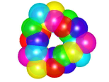
Figure 9: Six-component string ${\tt X}$ (hexaplet) formed of the unlike-charged tripole pairs spinning around their common ring-closed axis. Unlike Fig.8, where each colour charge is chown with its trajectory along the ring axis, the diagram above shows a “snap-shot” ( instantaneous configuration) of the charges constituting the hexaplet.

7 Combinations of closed strings and tripoles

The particles ${\tt Y}$, ${\tt X}$, as well as the $\triangle$-shaped tripoles, are similar to each other and can combine because of short-range forces caused by the residual chromaticism (known as gluonic van der Waals forces) of these structures. By considering spatial configurations of colour-charges in a pair of ring-closed structures, say ${\tt XX}$, ${\tt YY}$, or ${\tt XY}$, one can note that the sign of the van der Waals force depends on the particle helicities. Let us take a pair of like-charged ${\tt Y}$-particles with opposite helicities:

$${\tt Y}^{+}_{\upharpoonright}=\begin{bmatrix}\begin{turn}{-180.0}\raisebox{-7.19025pt}{\begin{turn}{-180.0}\raisebox{-7.19025pt}{ {\begin{turn}{-180.0}\raisebox{-7.19025pt}{\begin{turn}{-180.0}\raisebox{-7.19025pt}{$\triangle$}\end{turn}}\end{turn}}\raisebox{1.29167pt}{\tiny\begin{turn}{-180.0}\raisebox{-3.59512pt}{\begin{turn}{-180.0}\raisebox{-3.59512pt}{$+$}\end{turn}}\end{turn}}\raisebox{0.43057pt}{\tiny\begin{turn}{-180.0}\raisebox{-3.59512pt}{\begin{turn}{-180.0}\raisebox{-3.59512pt}{$\blacktriangle$}\end{turn}}\end{turn}} \hskip 0.86108pt}\end{turn}}\end{turn}\\ \begin{turn}{-180.0}\raisebox{-7.19025pt}{\begin{turn}{-180.0}\raisebox{-7.19025pt}{ {\begin{turn}{-180.0}\raisebox{-7.19025pt}{\begin{turn}{-180.0}\raisebox{-7.19025pt}{$\triangle$}\end{turn}}\end{turn}}\raisebox{0.86108pt}{\tiny\begin{turn}{-180.0}\raisebox{-3.59512pt}{\begin{turn}{-180.0}\raisebox{-3.59512pt}{$+$}\end{turn}}\end{turn}}\raisebox{4.30554pt}{\tiny\begin{turn}{-180.0}\raisebox{-3.59512pt}{\begin{turn}{-180.0}\raisebox{-3.59512pt}{$\blacktriangle$}\end{turn}}\end{turn}}\hskip 2.15277pt}\end{turn}}\end{turn}\\ \begin{turn}{-180.0}\raisebox{-7.19025pt}{\begin{turn}{-180.0}\raisebox{-7.19025pt}{ {\begin{turn}{-180.0}\raisebox{-7.19025pt}{\begin{turn}{-180.0}\raisebox{-7.19025pt}{$\triangle$}\end{turn}}\end{turn}}\raisebox{1.07639pt}{\tiny\begin{turn}{-180.0}\raisebox{-3.59512pt}{\begin{turn}{-180.0}\raisebox{-3.59512pt}{$+$}\end{turn}}\end{turn}}\raisebox{0.43057pt}{\tiny\begin{turn}{-180.0}\raisebox{-3.59512pt}{\begin{turn}{-180.0}\raisebox{-3.59512pt}{$\blacktriangle$}\end{turn}}\end{turn}}\hskip 0.43057pt}\end{turn}}\end{turn}\end{bmatrix}^{\upharpoonright}\hskip 8.61108pt\text{and}\hskip 12.91663pt{\tt Y}^{+}_{\downharpoonright}=\begin{bmatrix}\begin{turn}{-180.0}\raisebox{-7.19025pt}{ {\begin{turn}{-180.0}\raisebox{-7.19025pt}{\begin{turn}{-180.0}\raisebox{-7.19025pt}{$\triangle$}\end{turn}}\end{turn}}\raisebox{1.29167pt}{\tiny\begin{turn}{-180.0}\raisebox{-3.59512pt}{\begin{turn}{-180.0}\raisebox{-3.59512pt}{$+$}\end{turn}}\end{turn}}\raisebox{0.43057pt}{\tiny\begin{turn}{-180.0}\raisebox{-3.59512pt}{\begin{turn}{-180.0}\raisebox{-3.59512pt}{$\blacktriangle$}\end{turn}}\end{turn}} \hskip 0.86108pt}\end{turn}\\ \begin{turn}{-180.0}\raisebox{-7.19025pt}{ {\begin{turn}{-180.0}\raisebox{-7.19025pt}{\begin{turn}{-180.0}\raisebox{-7.19025pt}{$\triangle$}\end{turn}}\end{turn}}\raisebox{0.86108pt}{\tiny\begin{turn}{-180.0}\raisebox{-3.59512pt}{\begin{turn}{-180.0}\raisebox{-3.59512pt}{$+$}\end{turn}}\end{turn}}\raisebox{4.30554pt}{\tiny\begin{turn}{-180.0}\raisebox{-3.59512pt}{\begin{turn}{-180.0}\raisebox{-3.59512pt}{$\blacktriangle$}\end{turn}}\end{turn}}\hskip 2.15277pt}\end{turn}\\ \begin{turn}{-180.0}\raisebox{-7.19025pt}{ {\begin{turn}{-180.0}\raisebox{-7.19025pt}{\begin{turn}{-180.0}\raisebox{-7.19025pt}{$\triangle$}\end{turn}}\end{turn}}\raisebox{1.07639pt}{\tiny\begin{turn}{-180.0}\raisebox{-3.59512pt}{\begin{turn}{-180.0}\raisebox{-3.59512pt}{$+$}\end{turn}}\end{turn}}\raisebox{0.43057pt}{\tiny\begin{turn}{-180.0}\raisebox{-3.59512pt}{\begin{turn}{-180.0}\raisebox{-3.59512pt}{$\blacktriangle$}\end{turn}}\end{turn}}\hskip 0.43057pt}\end{turn}\end{bmatrix}_{\downharpoonright}\hskip 8.61108pt.$$ (47)

Let us assume that the rotational and oscillatory frequencies and phases of these particles are synchronised. In this regime the mutual orientation of the particle constituents remains always the same, which would simplify the analysis of such a combined system. The systems with no correlation between their moving constituents are not solvable in principle. Then, a probabilistic approach in the description of such systems would be more appropriate.

Note that in the representation (47) we mark the first component of each structure with the symbols $\upharpoonright$ and $\downharpoonright$ (denoting the clockwise and anticlockwise rotations, respectively) – to avoid possible confusion in the direction of rotation (these marks are not necessary in the case of a three-dimensional representation, as seen in Fig.6a).

The $\triangle$-shaped tripoles – the components of the structure ${\tt Y}^{+}_{\upharpoonright}{\tt Y}^{+}_{\downharpoonright}$ – are grouped in pairs and pair-wisely rotated by the position angle $\zeta=\pi$, which corresponds to the attractive force between them [see Fig.3(b) for $\rho>2\rho_{\circ}$]. Thus, besides the usual repulsive force between like-charges, the structure (47) has an additional – attractive – force between its componets:

$$\overset{\Leftarrow}{\begin{bmatrix}\begin{turn}{-180.0}\raisebox{-7.19025pt}{\begin{turn}{-180.0}\raisebox{-7.19025pt}{ {\begin{turn}{-180.0}\raisebox{-7.19025pt}{\begin{turn}{-180.0}\raisebox{-7.19025pt}{$\triangle$}\end{turn}}\end{turn}}\raisebox{1.29167pt}{\tiny\begin{turn}{-180.0}\raisebox{-3.59512pt}{\begin{turn}{-180.0}\raisebox{-3.59512pt}{$+$}\end{turn}}\end{turn}}\raisebox{0.43057pt}{\tiny\begin{turn}{-180.0}\raisebox{-3.59512pt}{\begin{turn}{-180.0}\raisebox{-3.59512pt}{$\blacktriangle$}\end{turn}}\end{turn}} \hskip 0.86108pt}\end{turn}}\end{turn}\\ \begin{turn}{-180.0}\raisebox{-7.19025pt}{\begin{turn}{-180.0}\raisebox{-7.19025pt}{ {\begin{turn}{-180.0}\raisebox{-7.19025pt}{\begin{turn}{-180.0}\raisebox{-7.19025pt}{$\triangle$}\end{turn}}\end{turn}}\raisebox{0.86108pt}{\tiny\begin{turn}{-180.0}\raisebox{-3.59512pt}{\begin{turn}{-180.0}\raisebox{-3.59512pt}{$+$}\end{turn}}\end{turn}}\raisebox{4.30554pt}{\tiny\begin{turn}{-180.0}\raisebox{-3.59512pt}{\begin{turn}{-180.0}\raisebox{-3.59512pt}{$\blacktriangle$}\end{turn}}\end{turn}}\hskip 2.15277pt}\end{turn}}\end{turn}\\ \begin{turn}{-180.0}\raisebox{-7.19025pt}{\begin{turn}{-180.0}\raisebox{-7.19025pt}{ {\begin{turn}{-180.0}\raisebox{-7.19025pt}{\begin{turn}{-180.0}\raisebox{-7.19025pt}{$\triangle$}\end{turn}}\end{turn}}\raisebox{1.07639pt}{\tiny\begin{turn}{-180.0}\raisebox{-3.59512pt}{\begin{turn}{-180.0}\raisebox{-3.59512pt}{$+$}\end{turn}}\end{turn}}\raisebox{0.43057pt}{\tiny\begin{turn}{-180.0}\raisebox{-3.59512pt}{\begin{turn}{-180.0}\raisebox{-3.59512pt}{$\blacktriangle$}\end{turn}}\end{turn}}\hskip 0.43057pt}\end{turn}}\end{turn}\end{bmatrix}^{\upharpoonright}}\begin{matrix}&\rightarrow&\leftarrow\\ &\rightarrow&\leftarrow\\ &\rightarrow&\leftarrow\end{matrix}\overset{\Rightarrow}{\begin{bmatrix}\begin{turn}{-180.0}\raisebox{-7.19025pt}{ {\begin{turn}{-180.0}\raisebox{-7.19025pt}{\begin{turn}{-180.0}\raisebox{-7.19025pt}{$\triangle$}\end{turn}}\end{turn}}\raisebox{1.29167pt}{\tiny\begin{turn}{-180.0}\raisebox{-3.59512pt}{\begin{turn}{-180.0}\raisebox{-3.59512pt}{$+$}\end{turn}}\end{turn}}\raisebox{0.43057pt}{\tiny\begin{turn}{-180.0}\raisebox{-3.59512pt}{\begin{turn}{-180.0}\raisebox{-3.59512pt}{$\blacktriangle$}\end{turn}}\end{turn}} \hskip 0.86108pt}\end{turn}\\ \begin{turn}{-180.0}\raisebox{-7.19025pt}{ {\begin{turn}{-180.0}\raisebox{-7.19025pt}{\begin{turn}{-180.0}\raisebox{-7.19025pt}{$\triangle$}\end{turn}}\end{turn}}\raisebox{0.86108pt}{\tiny\begin{turn}{-180.0}\raisebox{-3.59512pt}{\begin{turn}{-180.0}\raisebox{-3.59512pt}{$+$}\end{turn}}\end{turn}}\raisebox{4.30554pt}{\tiny\begin{turn}{-180.0}\raisebox{-3.59512pt}{\begin{turn}{-180.0}\raisebox{-3.59512pt}{$\blacktriangle$}\end{turn}}\end{turn}}\hskip 2.15277pt}\end{turn}\\ \begin{turn}{-180.0}\raisebox{-7.19025pt}{ {\begin{turn}{-180.0}\raisebox{-7.19025pt}{\begin{turn}{-180.0}\raisebox{-7.19025pt}{$\triangle$}\end{turn}}\end{turn}}\raisebox{1.07639pt}{\tiny\begin{turn}{-180.0}\raisebox{-3.59512pt}{\begin{turn}{-180.0}\raisebox{-3.59512pt}{$+$}\end{turn}}\end{turn}}\raisebox{0.43057pt}{\tiny\begin{turn}{-180.0}\raisebox{-3.59512pt}{\begin{turn}{-180.0}\raisebox{-3.59512pt}{$\blacktriangle$}\end{turn}}\end{turn}}\hskip 0.43057pt}\end{turn}\end{bmatrix}_{\downharpoonright}}~{}.$$ (48)

This implies the possibility of an equilibrium state (merger) of the pair, provided that there are no external forces and that the relative momenta of ${\tt Y}^{+}_{\upharpoonright}$ and ${\tt Y}^{+}_{\downharpoonright}$ are small enough. In this (entangled) state the orientation of the two particles is mutually dependent, which corresponds to the local minumum of the combined effective potential of the structure.

In the case of like-helicities, two of the three triplet pairs have the position angle $\zeta=\pi/6$ between the constititing tripoles, which would cause their repulsion from each other:

$$\begin{matrix}~{}\\ \leftarrow\\ \leftarrow\end{matrix}\overset{\Leftarrow}{\begin{bmatrix}\begin{turn}{-180.0}\raisebox{-7.19025pt}{\begin{turn}{-180.0}\raisebox{-7.19025pt}{ {\begin{turn}{-180.0}\raisebox{-7.19025pt}{\begin{turn}{-180.0}\raisebox{-7.19025pt}{$\triangle$}\end{turn}}\end{turn}}\raisebox{1.29167pt}{\tiny\begin{turn}{-180.0}\raisebox{-3.59512pt}{\begin{turn}{-180.0}\raisebox{-3.59512pt}{$+$}\end{turn}}\end{turn}}\raisebox{0.43057pt}{\tiny\begin{turn}{-180.0}\raisebox{-3.59512pt}{\begin{turn}{-180.0}\raisebox{-3.59512pt}{$\blacktriangle$}\end{turn}}\end{turn}} \hskip 0.86108pt}\end{turn}}\end{turn}\\ \begin{turn}{-180.0}\raisebox{-7.19025pt}{\begin{turn}{-180.0}\raisebox{-7.19025pt}{ {\begin{turn}{-180.0}\raisebox{-7.19025pt}{\begin{turn}{-180.0}\raisebox{-7.19025pt}{$\triangle$}\end{turn}}\end{turn}}\raisebox{0.86108pt}{\tiny\begin{turn}{-180.0}\raisebox{-3.59512pt}{\begin{turn}{-180.0}\raisebox{-3.59512pt}{$+$}\end{turn}}\end{turn}}\raisebox{4.30554pt}{\tiny\begin{turn}{-180.0}\raisebox{-3.59512pt}{\begin{turn}{-180.0}\raisebox{-3.59512pt}{$\blacktriangle$}\end{turn}}\end{turn}}\hskip 2.15277pt}\end{turn}}\end{turn}\\ \begin{turn}{-180.0}\raisebox{-7.19025pt}{\begin{turn}{-180.0}\raisebox{-7.19025pt}{ {\begin{turn}{-180.0}\raisebox{-7.19025pt}{\begin{turn}{-180.0}\raisebox{-7.19025pt}{$\triangle$}\end{turn}}\end{turn}}\raisebox{1.07639pt}{\tiny\begin{turn}{-180.0}\raisebox{-3.59512pt}{\begin{turn}{-180.0}\raisebox{-3.59512pt}{$+$}\end{turn}}\end{turn}}\raisebox{0.43057pt}{\tiny\begin{turn}{-180.0}\raisebox{-3.59512pt}{\begin{turn}{-180.0}\raisebox{-3.59512pt}{$\blacktriangle$}\end{turn}}\end{turn}}\hskip 0.43057pt}\end{turn}}\end{turn}\end{bmatrix}^{\upharpoonright}}\begin{matrix}&\rightarrow&\leftarrow\\ &~{}&~{}\\ &~{}&~{}\end{matrix}\overset{\Rightarrow}{\begin{bmatrix}\begin{turn}{-180.0}\raisebox{-7.19025pt}{ {\begin{turn}{-180.0}\raisebox{-7.19025pt}{\begin{turn}{-180.0}\raisebox{-7.19025pt}{$\triangle$}\end{turn}}\end{turn}}\raisebox{1.29167pt}{\tiny\begin{turn}{-180.0}\raisebox{-3.59512pt}{\begin{turn}{-180.0}\raisebox{-3.59512pt}{$+$}\end{turn}}\end{turn}}\raisebox{0.43057pt}{\tiny\begin{turn}{-180.0}\raisebox{-3.59512pt}{\begin{turn}{-180.0}\raisebox{-3.59512pt}{$\blacktriangle$}\end{turn}}\end{turn}} \hskip 0.86108pt}\end{turn}\\ \begin{turn}{-180.0}\raisebox{-7.19025pt}{ {\begin{turn}{-180.0}\raisebox{-7.19025pt}{\begin{turn}{-180.0}\raisebox{-7.19025pt}{$\triangle$}\end{turn}}\end{turn}}\raisebox{1.07639pt}{\tiny\begin{turn}{-180.0}\raisebox{-3.59512pt}{\begin{turn}{-180.0}\raisebox{-3.59512pt}{$+$}\end{turn}}\end{turn}}\raisebox{0.43057pt}{\tiny\begin{turn}{-180.0}\raisebox{-3.59512pt}{\begin{turn}{-180.0}\raisebox{-3.59512pt}{$\blacktriangle$}\end{turn}}\end{turn}}\hskip 0.43057pt}\end{turn}\\ \begin{turn}{-180.0}\raisebox{-7.19025pt}{ {\begin{turn}{-180.0}\raisebox{-7.19025pt}{\begin{turn}{-180.0}\raisebox{-7.19025pt}{$\triangle$}\end{turn}}\end{turn}}\raisebox{0.86108pt}{\tiny\begin{turn}{-180.0}\raisebox{-3.59512pt}{\begin{turn}{-180.0}\raisebox{-3.59512pt}{$+$}\end{turn}}\end{turn}}\raisebox{4.30554pt}{\tiny\begin{turn}{-180.0}\raisebox{-3.59512pt}{\begin{turn}{-180.0}\raisebox{-3.59512pt}{$\blacktriangle$}\end{turn}}\end{turn}}\hskip 2.15277pt}\end{turn}\end{bmatrix}_{\upharpoonright}}\begin{matrix}~{}\\ &\rightarrow\\ &\rightarrow\end{matrix}\hskip 12.91663pt.$$ (49)

This inhibits the entanglement of the particles with like-helicities. It is noteworthy that the pattern of attraction and repulsion in the diagrams (48)-(49) coheres with (and probably explains the origin of) the Pauli exclusion principle.

In the merger (48) the Y-particles are joined co-axially (pole-to-pole) to each other. But they could also be coupled side-by-side (laterally) provided that their vectors of angular momenta are aligned, for instance, because of some external magnetic field. In this case, the pattern of attraction for the opposite helicities and repulsion for the like-helicities will also be reproduced. This means that every colour charge would tend to occupy a position always in front of two other colour-charges, complementary to the first one. The structure with the laterally coupled Y-particles can grow (in principle, indefinitely) as a “two-dimensional” hexagonal lattice, as shown in Fig.10.

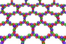
Figure 10: A “snap-shot” of the hexagonal lattice formed by the side-by-side (off-axial) coupling of the triplets ${\tt Y}$.

Note that the lattice is shown here as a “stand-still” structure, although in reality its constituents are spinning (see Fig.8). The stand-still representation is possible because of the above mentioned synchronisation of frequencies and phases between neighbouring Y-particles.

The two-dimensional infinite lattice, Fig.10, can hardly be stable. But it can be closed into more stable configurations with lower energies, such as a hollow tube (Fig.11a), which can further be closed in a torus (Fig.11b). The latter would be stable because its further closure is unlikely (as with any other ring-structure). The minimal torus can be formed of 108 ${\tt Y}$-triplets (${\tt T}_{108}$) or, alternatively, of 54 pairs ${\tt Y}^{+}{\tt Y}^{-}={\tt Y}^{\circ}$. In the latter case the particle ${\tt T}_{108}$ will be electrically neutral.

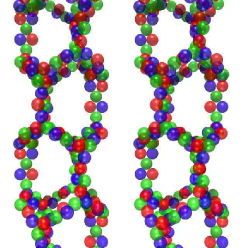
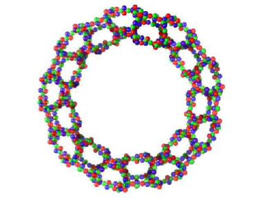
Figure 11: (a) Hexagonal lattice of ${\tt Y}$-particles closed in a hollow tube; (b) the tube is further closed in a minimal-energy torus ${\tt T}_{108}$ of 108 ${\tt Y}$-particles (54 neutral pairs ${\tt Y}^{+}{\tt Y}^{-}$).

Another possibility to form a stable neutral structure of the triplets ${\tt Y}$ is the spherical closure of the lattice, as shown in Fig.12. The minimal number of ${\tt Y}$-particles that can combine in a hollow sphere is eight (or, respectively, four pairs of the oppositely charged ${\tt Y}^{+}$ and ${\tt Y}^{-}$ particles).

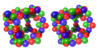
Figure 12: Spherically-closed structure ${\tt S}_{8}$ composed of eight triplets Y (four neutral pairs ${\tt Y}^{+}{\tt Y}^{-}$).

Analysing the structural diagrams for the hexaplets ${\tt X}$ one will find that the dispersive (van der Vaals) force between ${\tt X}_{\downharpoonright}$ and ${\tt X}_{\upharpoonright}$ is attractive and between ${\tt X}_{\downharpoonright}$ and ${\tt X}_{\downharpoonright}$ (or ${\tt X}_{\upharpoonright}$ and ${\tt X}_{\upharpoonright}$) – repulsive. However, in the case of a hexaplet combined with a triplet (${\tt XY}$) the pattern of attraction and repulsion is inversed: the local chromaticism of ${\tt X}$ would be affine (attractive) to that of ${\tt Y}$ only if both particles have like-helicities.

For the pairs of unlike-charged particles, ${\tt Y}^{+}$ and ${\tt Y}^{-}$, the pattern of attraction and repulsion is similar to (48)-(49), with the only difference that, in addition to this pattern, there exists the conventional attractive force between opposite charges:

$${\tt Y}^{+}_{\upharpoonright}+{\tt Y}^{-}_{\downharpoonright}=\hskip 4.30554pt\overset{\Rightarrow}{\begin{bmatrix}\begin{turn}{-180.0}\raisebox{-7.19025pt}{\begin{turn}{-180.0}\raisebox{-7.19025pt}{ {\begin{turn}{-180.0}\raisebox{-7.19025pt}{\begin{turn}{-180.0}\raisebox{-7.19025pt}{$\triangle$}\end{turn}}\end{turn}}\raisebox{1.29167pt}{\tiny\begin{turn}{-180.0}\raisebox{-3.59512pt}{\begin{turn}{-180.0}\raisebox{-3.59512pt}{$+$}\end{turn}}\end{turn}}\raisebox{0.43057pt}{\tiny\begin{turn}{-180.0}\raisebox{-3.59512pt}{\begin{turn}{-180.0}\raisebox{-3.59512pt}{$\blacktriangle$}\end{turn}}\end{turn}} \hskip 0.86108pt}\end{turn}}\end{turn}\\ \begin{turn}{-180.0}\raisebox{-7.19025pt}{\begin{turn}{-180.0}\raisebox{-7.19025pt}{ {\begin{turn}{-180.0}\raisebox{-7.19025pt}{\begin{turn}{-180.0}\raisebox{-7.19025pt}{$\triangle$}\end{turn}}\end{turn}}\raisebox{0.86108pt}{\tiny\begin{turn}{-180.0}\raisebox{-3.59512pt}{\begin{turn}{-180.0}\raisebox{-3.59512pt}{$+$}\end{turn}}\end{turn}}\raisebox{4.30554pt}{\tiny\begin{turn}{-180.0}\raisebox{-3.59512pt}{\begin{turn}{-180.0}\raisebox{-3.59512pt}{$\blacktriangle$}\end{turn}}\end{turn}}\hskip 2.15277pt}\end{turn}}\end{turn}\\ \begin{turn}{-180.0}\raisebox{-7.19025pt}{\begin{turn}{-180.0}\raisebox{-7.19025pt}{ {\begin{turn}{-180.0}\raisebox{-7.19025pt}{\begin{turn}{-180.0}\raisebox{-7.19025pt}{$\triangle$}\end{turn}}\end{turn}}\raisebox{1.07639pt}{\tiny\begin{turn}{-180.0}\raisebox{-3.59512pt}{\begin{turn}{-180.0}\raisebox{-3.59512pt}{$+$}\end{turn}}\end{turn}}\raisebox{0.43057pt}{\tiny\begin{turn}{-180.0}\raisebox{-3.59512pt}{\begin{turn}{-180.0}\raisebox{-3.59512pt}{$\blacktriangle$}\end{turn}}\end{turn}}\hskip 0.43057pt}\end{turn}}\end{turn}\end{bmatrix}^{\upharpoonright}}\begin{matrix}&\rightarrow&\leftarrow\\ &\rightarrow&\leftarrow\\ &\rightarrow&\leftarrow\end{matrix}\overset{\Leftarrow}{\begin{bmatrix}\begin{turn}{-180.0}\raisebox{-7.19025pt}{ {\begin{turn}{-180.0}\raisebox{-7.19025pt}{\begin{turn}{-180.0}\raisebox{-7.19025pt}{$\triangle$}\end{turn}}\end{turn}}\raisebox{1.29167pt}{\tiny\begin{turn}{-180.0}\raisebox{-3.59512pt}{\begin{turn}{-180.0}\raisebox{-3.59512pt}{$-$}\end{turn}}\end{turn}}\raisebox{0.43057pt}{\tiny\begin{turn}{-180.0}\raisebox{-3.59512pt}{\begin{turn}{-180.0}\raisebox{-3.59512pt}{$\blacktriangle$}\end{turn}}\end{turn}} \hskip 0.86108pt}\end{turn}\\ \begin{turn}{-180.0}\raisebox{-7.19025pt}{ {\begin{turn}{-180.0}\raisebox{-7.19025pt}{\begin{turn}{-180.0}\raisebox{-7.19025pt}{$\triangle$}\end{turn}}\end{turn}}\raisebox{0.86108pt}{\tiny\begin{turn}{-180.0}\raisebox{-3.59512pt}{\begin{turn}{-180.0}\raisebox{-3.59512pt}{$-$}\end{turn}}\end{turn}}\raisebox{4.30554pt}{\tiny\begin{turn}{-180.0}\raisebox{-3.59512pt}{\begin{turn}{-180.0}\raisebox{-3.59512pt}{$\blacktriangle$}\end{turn}}\end{turn}}\hskip 2.15277pt}\end{turn}\\ \begin{turn}{-180.0}\raisebox{-7.19025pt}{ {\begin{turn}{-180.0}\raisebox{-7.19025pt}{\begin{turn}{-180.0}\raisebox{-7.19025pt}{$\triangle$}\end{turn}}\end{turn}}\raisebox{1.07639pt}{\tiny\begin{turn}{-180.0}\raisebox{-3.59512pt}{\begin{turn}{-180.0}\raisebox{-3.59512pt}{$-$}\end{turn}}\end{turn}}\raisebox{0.43057pt}{\tiny\begin{turn}{-180.0}\raisebox{-3.59512pt}{\begin{turn}{-180.0}\raisebox{-3.59512pt}{$\blacktriangle$}\end{turn}}\end{turn}}\hskip 0.43057pt}\end{turn}\end{bmatrix}_{\downharpoonright}}~{}$$ (50)

$${\tt Y}^{+}_{\upharpoonright}+{\tt Y}^{-}_{\upharpoonright}=\hskip 4.30554pt\begin{matrix}~{}\\ \leftarrow\\ \leftarrow\end{matrix}\overset{\Rightarrow}{\begin{bmatrix}\begin{turn}{-180.0}\raisebox{-7.19025pt}{\begin{turn}{-180.0}\raisebox{-7.19025pt}{ {\begin{turn}{-180.0}\raisebox{-7.19025pt}{\begin{turn}{-180.0}\raisebox{-7.19025pt}{$\triangle$}\end{turn}}\end{turn}}\raisebox{1.29167pt}{\tiny\begin{turn}{-180.0}\raisebox{-3.59512pt}{\begin{turn}{-180.0}\raisebox{-3.59512pt}{$+$}\end{turn}}\end{turn}}\raisebox{0.43057pt}{\tiny\begin{turn}{-180.0}\raisebox{-3.59512pt}{\begin{turn}{-180.0}\raisebox{-3.59512pt}{$\blacktriangle$}\end{turn}}\end{turn}} \hskip 0.86108pt}\end{turn}}\end{turn}\\ \begin{turn}{-180.0}\raisebox{-7.19025pt}{\begin{turn}{-180.0}\raisebox{-7.19025pt}{ {\begin{turn}{-180.0}\raisebox{-7.19025pt}{\begin{turn}{-180.0}\raisebox{-7.19025pt}{$\triangle$}\end{turn}}\end{turn}}\raisebox{0.86108pt}{\tiny\begin{turn}{-180.0}\raisebox{-3.59512pt}{\begin{turn}{-180.0}\raisebox{-3.59512pt}{$+$}\end{turn}}\end{turn}}\raisebox{4.30554pt}{\tiny\begin{turn}{-180.0}\raisebox{-3.59512pt}{\begin{turn}{-180.0}\raisebox{-3.59512pt}{$\blacktriangle$}\end{turn}}\end{turn}}\hskip 2.15277pt}\end{turn}}\end{turn}\\ \begin{turn}{-180.0}\raisebox{-7.19025pt}{\begin{turn}{-180.0}\raisebox{-7.19025pt}{ {\begin{turn}{-180.0}\raisebox{-7.19025pt}{\begin{turn}{-180.0}\raisebox{-7.19025pt}{$\triangle$}\end{turn}}\end{turn}}\raisebox{1.07639pt}{\tiny\begin{turn}{-180.0}\raisebox{-3.59512pt}{\begin{turn}{-180.0}\raisebox{-3.59512pt}{$+$}\end{turn}}\end{turn}}\raisebox{0.43057pt}{\tiny\begin{turn}{-180.0}\raisebox{-3.59512pt}{\begin{turn}{-180.0}\raisebox{-3.59512pt}{$\blacktriangle$}\end{turn}}\end{turn}}\hskip 0.43057pt}\end{turn}}\end{turn}\end{bmatrix}^{\upharpoonright}}\begin{matrix}&\rightarrow&\leftarrow\\ &~{}&~{}\\ &~{}&~{}\end{matrix}\overset{\Leftarrow}{\begin{bmatrix}\begin{turn}{-180.0}\raisebox{-7.19025pt}{ {\begin{turn}{-180.0}\raisebox{-7.19025pt}{\begin{turn}{-180.0}\raisebox{-7.19025pt}{$\triangle$}\end{turn}}\end{turn}}\raisebox{1.29167pt}{\tiny\begin{turn}{-180.0}\raisebox{-3.59512pt}{\begin{turn}{-180.0}\raisebox{-3.59512pt}{$-$}\end{turn}}\end{turn}}\raisebox{0.43057pt}{\tiny\begin{turn}{-180.0}\raisebox{-3.59512pt}{\begin{turn}{-180.0}\raisebox{-3.59512pt}{$\blacktriangle$}\end{turn}}\end{turn}} \hskip 0.86108pt}\end{turn}\\ \begin{turn}{-180.0}\raisebox{-7.19025pt}{ {\begin{turn}{-180.0}\raisebox{-7.19025pt}{\begin{turn}{-180.0}\raisebox{-7.19025pt}{$\triangle$}\end{turn}}\end{turn}}\raisebox{1.07639pt}{\tiny\begin{turn}{-180.0}\raisebox{-3.59512pt}{\begin{turn}{-180.0}\raisebox{-3.59512pt}{$-$}\end{turn}}\end{turn}}\raisebox{0.43057pt}{\tiny\begin{turn}{-180.0}\raisebox{-3.59512pt}{\begin{turn}{-180.0}\raisebox{-3.59512pt}{$\blacktriangle$}\end{turn}}\end{turn}}\hskip 0.43057pt}\end{turn}\\ \begin{turn}{-180.0}\raisebox{-7.19025pt}{ {\begin{turn}{-180.0}\raisebox{-7.19025pt}{\begin{turn}{-180.0}\raisebox{-7.19025pt}{$\triangle$}\end{turn}}\end{turn}}\raisebox{0.86108pt}{\tiny\begin{turn}{-180.0}\raisebox{-3.59512pt}{\begin{turn}{-180.0}\raisebox{-3.59512pt}{$-$}\end{turn}}\end{turn}}\raisebox{4.30554pt}{\tiny\begin{turn}{-180.0}\raisebox{-3.59512pt}{\begin{turn}{-180.0}\raisebox{-3.59512pt}{$\blacktriangle$}\end{turn}}\end{turn}}\hskip 2.15277pt}\end{turn}\end{bmatrix}_{\upharpoonright}}\begin{matrix}~{}\\ &\rightarrow\\ &\rightarrow\end{matrix}~{}.$$ (51)

The potential of the system (51) has a repulsive inner and attractive outer region, whereas both the inner and outer regions of the potential of the system (50) are attractive. As a result, two unlike-charged ${\tt Y}$-particles would tend to merge, reaching an equilibrium (the neutral merger ${\tt Y}^{\circ}$ ) state between the constituents of both particles, which is possible if we suppose that the dynamics of the system is suppressed (say, by an external magnetic field). Actually, this state:

$${\tt Y}^{\circ}=\hskip 4.30554pt\begin{bmatrix}\begin{turn}{-180.0}\raisebox{-7.19025pt}{\begin{turn}{-180.0}\raisebox{-7.19025pt}{ {\begin{turn}{-180.0}\raisebox{-7.19025pt}{\begin{turn}{-180.0}\raisebox{-7.19025pt}{$\triangle$}\end{turn}}\end{turn}}\raisebox{1.29167pt}{\tiny\begin{turn}{-180.0}\raisebox{-3.59512pt}{\begin{turn}{-180.0}\raisebox{-3.59512pt}{$+$}\end{turn}}\end{turn}}\raisebox{0.43057pt}{\tiny\begin{turn}{-180.0}\raisebox{-3.59512pt}{\begin{turn}{-180.0}\raisebox{-3.59512pt}{$\blacktriangle$}\end{turn}}\end{turn}} \hskip 0.86108pt}\end{turn}}\end{turn}\begin{turn}{-180.0}\raisebox{-7.19025pt}{ {\begin{turn}{-180.0}\raisebox{-7.19025pt}{\begin{turn}{-180.0}\raisebox{-7.19025pt}{$\triangle$}\end{turn}}\end{turn}}\raisebox{1.29167pt}{\tiny\begin{turn}{-180.0}\raisebox{-3.59512pt}{\begin{turn}{-180.0}\raisebox{-3.59512pt}{$-$}\end{turn}}\end{turn}}\raisebox{0.43057pt}{\tiny\begin{turn}{-180.0}\raisebox{-3.59512pt}{\begin{turn}{-180.0}\raisebox{-3.59512pt}{$\blacktriangle$}\end{turn}}\end{turn}} \hskip 0.86108pt}\end{turn}\\ \begin{turn}{-180.0}\raisebox{-7.19025pt}{\begin{turn}{-180.0}\raisebox{-7.19025pt}{ {\begin{turn}{-180.0}\raisebox{-7.19025pt}{\begin{turn}{-180.0}\raisebox{-7.19025pt}{$\triangle$}\end{turn}}\end{turn}}\raisebox{0.86108pt}{\tiny\begin{turn}{-180.0}\raisebox{-3.59512pt}{\begin{turn}{-180.0}\raisebox{-3.59512pt}{$+$}\end{turn}}\end{turn}}\raisebox{4.30554pt}{\tiny\begin{turn}{-180.0}\raisebox{-3.59512pt}{\begin{turn}{-180.0}\raisebox{-3.59512pt}{$\blacktriangle$}\end{turn}}\end{turn}}\hskip 2.15277pt}\end{turn}}\end{turn}\begin{turn}{-180.0}\raisebox{-7.19025pt}{ {\begin{turn}{-180.0}\raisebox{-7.19025pt}{\begin{turn}{-180.0}\raisebox{-7.19025pt}{$\triangle$}\end{turn}}\end{turn}}\raisebox{0.86108pt}{\tiny\begin{turn}{-180.0}\raisebox{-3.59512pt}{\begin{turn}{-180.0}\raisebox{-3.59512pt}{$-$}\end{turn}}\end{turn}}\raisebox{4.30554pt}{\tiny\begin{turn}{-180.0}\raisebox{-3.59512pt}{\begin{turn}{-180.0}\raisebox{-3.59512pt}{$\blacktriangle$}\end{turn}}\end{turn}}\hskip 2.15277pt}\end{turn}\\ \begin{turn}{-180.0}\raisebox{-7.19025pt}{\begin{turn}{-180.0}\raisebox{-7.19025pt}{ {\begin{turn}{-180.0}\raisebox{-7.19025pt}{\begin{turn}{-180.0}\raisebox{-7.19025pt}{$\triangle$}\end{turn}}\end{turn}}\raisebox{1.07639pt}{\tiny\begin{turn}{-180.0}\raisebox{-3.59512pt}{\begin{turn}{-180.0}\raisebox{-3.59512pt}{$+$}\end{turn}}\end{turn}}\raisebox{0.43057pt}{\tiny\begin{turn}{-180.0}\raisebox{-3.59512pt}{\begin{turn}{-180.0}\raisebox{-3.59512pt}{$\blacktriangle$}\end{turn}}\end{turn}}\hskip 0.43057pt}\end{turn}}\end{turn}\begin{turn}{-180.0}\raisebox{-7.19025pt}{ {\begin{turn}{-180.0}\raisebox{-7.19025pt}{\begin{turn}{-180.0}\raisebox{-7.19025pt}{$\triangle$}\end{turn}}\end{turn}}\raisebox{1.07639pt}{\tiny\begin{turn}{-180.0}\raisebox{-3.59512pt}{\begin{turn}{-180.0}\raisebox{-3.59512pt}{$-$}\end{turn}}\end{turn}}\raisebox{0.43057pt}{\tiny\begin{turn}{-180.0}\raisebox{-3.59512pt}{\begin{turn}{-180.0}\raisebox{-3.59512pt}{$\blacktriangle$}\end{turn}}\end{turn}}\hskip 0.43057pt}\end{turn}\end{bmatrix}=\begin{bmatrix}{\sf d}^{\circ}\\ {\sf d}^{\circ}\\ {\sf d}^{\circ}\end{bmatrix}~{}$$ (52)

consists of three neutral doublets ${\sf d}^{\circ}$ (33) joined together by their residual chromofields. The ground-state energy (mass) of this neutral system will correspond to the masses of its two constituents, ${\tt Y}^{+}$ and ${\tt Y}^{-}$, less the binding energy between them, $\hat{E}_{{\tt Y}^{+}{\tt Y}^{-}}$:

$$m_{{\tt Y}^{\circ}}\approx 2m_{\tt Y}-\hat{E}_{{\tt Y}^{+}{\tt Y}^{-}}<18~{}[m_{\circ}].$$ (53)

The bonds between these three doublets ${\sf d}^{\circ}$ must be weak because there is no attractive electric force between neutral particles, and the doublets here are joined only by their residual chromofields. Thus, even small perturbations would cause this structure to desintegrate into three neutral doublets. The corresponding reaction can be written as

$${\tt Y}^{+}_{\upharpoonright}+{\tt Y}^{-}_{\downharpoonright}=\hskip 4.30554pt\overset{\Rightarrow}{\begin{bmatrix}\begin{turn}{-180.0}\raisebox{-7.19025pt}{\begin{turn}{-180.0}\raisebox{-7.19025pt}{ {\begin{turn}{-180.0}\raisebox{-7.19025pt}{\begin{turn}{-180.0}\raisebox{-7.19025pt}{$\triangle$}\end{turn}}\end{turn}}\raisebox{1.29167pt}{\tiny\begin{turn}{-180.0}\raisebox{-3.59512pt}{\begin{turn}{-180.0}\raisebox{-3.59512pt}{$+$}\end{turn}}\end{turn}}\raisebox{0.43057pt}{\tiny\begin{turn}{-180.0}\raisebox{-3.59512pt}{\begin{turn}{-180.0}\raisebox{-3.59512pt}{$\blacktriangle$}\end{turn}}\end{turn}} \hskip 0.86108pt}\end{turn}}\end{turn}\\ \begin{turn}{-180.0}\raisebox{-7.19025pt}{\begin{turn}{-180.0}\raisebox{-7.19025pt}{ {\begin{turn}{-180.0}\raisebox{-7.19025pt}{\begin{turn}{-180.0}\raisebox{-7.19025pt}{$\triangle$}\end{turn}}\end{turn}}\raisebox{0.86108pt}{\tiny\begin{turn}{-180.0}\raisebox{-3.59512pt}{\begin{turn}{-180.0}\raisebox{-3.59512pt}{$+$}\end{turn}}\end{turn}}\raisebox{4.30554pt}{\tiny\begin{turn}{-180.0}\raisebox{-3.59512pt}{\begin{turn}{-180.0}\raisebox{-3.59512pt}{$\blacktriangle$}\end{turn}}\end{turn}}\hskip 2.15277pt}\end{turn}}\end{turn}\\ \begin{turn}{-180.0}\raisebox{-7.19025pt}{\begin{turn}{-180.0}\raisebox{-7.19025pt}{ {\begin{turn}{-180.0}\raisebox{-7.19025pt}{\begin{turn}{-180.0}\raisebox{-7.19025pt}{$\triangle$}\end{turn}}\end{turn}}\raisebox{1.07639pt}{\tiny\begin{turn}{-180.0}\raisebox{-3.59512pt}{\begin{turn}{-180.0}\raisebox{-3.59512pt}{$+$}\end{turn}}\end{turn}}\raisebox{0.43057pt}{\tiny\begin{turn}{-180.0}\raisebox{-3.59512pt}{\begin{turn}{-180.0}\raisebox{-3.59512pt}{$\blacktriangle$}\end{turn}}\end{turn}}\hskip 0.43057pt}\end{turn}}\end{turn}\end{bmatrix}^{\upharpoonright}}\begin{matrix}&\rightarrow&\leftarrow\\ &\rightarrow&\leftarrow\\ &\rightarrow&\leftarrow\end{matrix}\overset{\Leftarrow}{\begin{bmatrix}\begin{turn}{-180.0}\raisebox{-7.19025pt}{ {\begin{turn}{-180.0}\raisebox{-7.19025pt}{\begin{turn}{-180.0}\raisebox{-7.19025pt}{$\triangle$}\end{turn}}\end{turn}}\raisebox{1.29167pt}{\tiny\begin{turn}{-180.0}\raisebox{-3.59512pt}{\begin{turn}{-180.0}\raisebox{-3.59512pt}{$-$}\end{turn}}\end{turn}}\raisebox{0.43057pt}{\tiny\begin{turn}{-180.0}\raisebox{-3.59512pt}{\begin{turn}{-180.0}\raisebox{-3.59512pt}{$\blacktriangle$}\end{turn}}\end{turn}} \hskip 0.86108pt}\end{turn}\\ \begin{turn}{-180.0}\raisebox{-7.19025pt}{ {\begin{turn}{-180.0}\raisebox{-7.19025pt}{\begin{turn}{-180.0}\raisebox{-7.19025pt}{$\triangle$}\end{turn}}\end{turn}}\raisebox{0.86108pt}{\tiny\begin{turn}{-180.0}\raisebox{-3.59512pt}{\begin{turn}{-180.0}\raisebox{-3.59512pt}{$-$}\end{turn}}\end{turn}}\raisebox{4.30554pt}{\tiny\begin{turn}{-180.0}\raisebox{-3.59512pt}{\begin{turn}{-180.0}\raisebox{-3.59512pt}{$\blacktriangle$}\end{turn}}\end{turn}}\hskip 2.15277pt}\end{turn}\\ \begin{turn}{-180.0}\raisebox{-7.19025pt}{ {\begin{turn}{-180.0}\raisebox{-7.19025pt}{\begin{turn}{-180.0}\raisebox{-7.19025pt}{$\triangle$}\end{turn}}\end{turn}}\raisebox{1.07639pt}{\tiny\begin{turn}{-180.0}\raisebox{-3.59512pt}{\begin{turn}{-180.0}\raisebox{-3.59512pt}{$-$}\end{turn}}\end{turn}}\raisebox{0.43057pt}{\tiny\begin{turn}{-180.0}\raisebox{-3.59512pt}{\begin{turn}{-180.0}\raisebox{-3.59512pt}{$\blacktriangle$}\end{turn}}\end{turn}}\hskip 0.43057pt}\end{turn}\end{bmatrix}_{\downharpoonright}}~{}\longrightarrow~{}\begin{matrix}[\begin{turn}{-180.0}\raisebox{-7.19025pt}{\begin{turn}{-180.0}\raisebox{-7.19025pt}{ {\begin{turn}{-180.0}\raisebox{-7.19025pt}{\begin{turn}{-180.0}\raisebox{-7.19025pt}{$\triangle$}\end{turn}}\end{turn}}\raisebox{1.29167pt}{\tiny\begin{turn}{-180.0}\raisebox{-3.59512pt}{\begin{turn}{-180.0}\raisebox{-3.59512pt}{$+$}\end{turn}}\end{turn}}\raisebox{0.43057pt}{\tiny\begin{turn}{-180.0}\raisebox{-3.59512pt}{\begin{turn}{-180.0}\raisebox{-3.59512pt}{$\blacktriangle$}\end{turn}}\end{turn}} \hskip 0.86108pt}\end{turn}}\end{turn}\begin{turn}{-180.0}\raisebox{-7.19025pt}{ {\begin{turn}{-180.0}\raisebox{-7.19025pt}{\begin{turn}{-180.0}\raisebox{-7.19025pt}{$\triangle$}\end{turn}}\end{turn}}\raisebox{1.29167pt}{\tiny\begin{turn}{-180.0}\raisebox{-3.59512pt}{\begin{turn}{-180.0}\raisebox{-3.59512pt}{$-$}\end{turn}}\end{turn}}\raisebox{0.43057pt}{\tiny\begin{turn}{-180.0}\raisebox{-3.59512pt}{\begin{turn}{-180.0}\raisebox{-3.59512pt}{$\blacktriangle$}\end{turn}}\end{turn}} \hskip 0.86108pt}\end{turn}]={\sf d}^{\circ}\\ [\begin{turn}{-180.0}\raisebox{-7.19025pt}{\begin{turn}{-180.0}\raisebox{-7.19025pt}{ {\begin{turn}{-180.0}\raisebox{-7.19025pt}{\begin{turn}{-180.0}\raisebox{-7.19025pt}{$\triangle$}\end{turn}}\end{turn}}\raisebox{0.86108pt}{\tiny\begin{turn}{-180.0}\raisebox{-3.59512pt}{\begin{turn}{-180.0}\raisebox{-3.59512pt}{$+$}\end{turn}}\end{turn}}\raisebox{4.30554pt}{\tiny\begin{turn}{-180.0}\raisebox{-3.59512pt}{\begin{turn}{-180.0}\raisebox{-3.59512pt}{$\blacktriangle$}\end{turn}}\end{turn}}\hskip 2.15277pt}\end{turn}}\end{turn}\begin{turn}{-180.0}\raisebox{-7.19025pt}{ {\begin{turn}{-180.0}\raisebox{-7.19025pt}{\begin{turn}{-180.0}\raisebox{-7.19025pt}{$\triangle$}\end{turn}}\end{turn}}\raisebox{0.86108pt}{\tiny\begin{turn}{-180.0}\raisebox{-3.59512pt}{\begin{turn}{-180.0}\raisebox{-3.59512pt}{$-$}\end{turn}}\end{turn}}\raisebox{4.30554pt}{\tiny\begin{turn}{-180.0}\raisebox{-3.59512pt}{\begin{turn}{-180.0}\raisebox{-3.59512pt}{$\blacktriangle$}\end{turn}}\end{turn}}\hskip 2.15277pt}\end{turn}]={\sf d}^{\circ}\\ [\begin{turn}{-180.0}\raisebox{-7.19025pt}{\begin{turn}{-180.0}\raisebox{-7.19025pt}{ {\begin{turn}{-180.0}\raisebox{-7.19025pt}{\begin{turn}{-180.0}\raisebox{-7.19025pt}{$\triangle$}\end{turn}}\end{turn}}\raisebox{1.07639pt}{\tiny\begin{turn}{-180.0}\raisebox{-3.59512pt}{\begin{turn}{-180.0}\raisebox{-3.59512pt}{$+$}\end{turn}}\end{turn}}\raisebox{0.43057pt}{\tiny\begin{turn}{-180.0}\raisebox{-3.59512pt}{\begin{turn}{-180.0}\raisebox{-3.59512pt}{$\blacktriangle$}\end{turn}}\end{turn}}\hskip 0.43057pt}\end{turn}}\end{turn}\begin{turn}{-180.0}\raisebox{-7.19025pt}{ {\begin{turn}{-180.0}\raisebox{-7.19025pt}{\begin{turn}{-180.0}\raisebox{-7.19025pt}{$\triangle$}\end{turn}}\end{turn}}\raisebox{1.07639pt}{\tiny\begin{turn}{-180.0}\raisebox{-3.59512pt}{\begin{turn}{-180.0}\raisebox{-3.59512pt}{$-$}\end{turn}}\end{turn}}\raisebox{0.43057pt}{\tiny\begin{turn}{-180.0}\raisebox{-3.59512pt}{\begin{turn}{-180.0}\raisebox{-3.59512pt}{$\blacktriangle$}\end{turn}}\end{turn}}\hskip 0.43057pt}\end{turn}]={\sf d}^{\circ}\end{matrix}$$ (54)

or, in brief,

$${\tt Y}^{+}_{\upharpoonright}+{\tt Y}^{-}_{\downharpoonright}\overset{t_{\upharpoonright\downharpoonright}}{\longrightarrow}3{\sf d}^{\circ},$$ (55)

where $t_{\upharpoonright\downharpoonright}$ is the time, which is needed to complete the reaction. Alternatively, the particles ${\tt Y}^{+}_{\upharpoonright}$ and ${\tt Y}^{-}_{\downharpoonright}$ can separate without loosing their integrity, which would correspond to their elastic scattering.

In the system (51) of a pair of ${\tt Y}$-particles with like-helicities, two of three tripole-antitripole pairs have the position angles $\zeta=\pi/6$ corresponding to a repulsive force, which precludes direct merging of these components into neutral doublets. Instead, energetically, it is more economic for these two pairs of triplets to combine first into two charged doublets ${\sf d}^{+}$ and ${\sf d}^{-}$, Eq. (31). Only after that, these intermediate structures could merge and form a neutral system (35) ${\sf d}^{\circ}_{2}$:

$$\raisebox{-6.45831pt}{ \begin{turn}{-180.0}\raisebox{-7.19025pt}{\begin{turn}{-180.0}\raisebox{-7.19025pt}{ {\begin{turn}{-180.0}\raisebox{-7.19025pt}{\begin{turn}{-180.0}\raisebox{-7.19025pt}{$\triangle$}\end{turn}}\end{turn}}\raisebox{0.86108pt}{\tiny\begin{turn}{-180.0}\raisebox{-3.59512pt}{\begin{turn}{-180.0}\raisebox{-3.59512pt}{$+$}\end{turn}}\end{turn}}\raisebox{4.30554pt}{\tiny\begin{turn}{-180.0}\raisebox{-3.59512pt}{\begin{turn}{-180.0}\raisebox{-3.59512pt}{$\blacktriangle$}\end{turn}}\end{turn}}\hskip 2.15277pt}\end{turn}}\end{turn}\begin{turn}{-180.0}\raisebox{-7.19025pt}{\begin{turn}{-180.0}\raisebox{-7.19025pt}{ {\begin{turn}{-180.0}\raisebox{-7.19025pt}{\begin{turn}{-180.0}\raisebox{-7.19025pt}{$\triangle$}\end{turn}}\end{turn}}\raisebox{1.07639pt}{\tiny\begin{turn}{-180.0}\raisebox{-3.59512pt}{\begin{turn}{-180.0}\raisebox{-3.59512pt}{$+$}\end{turn}}\end{turn}}\raisebox{0.43057pt}{\tiny\begin{turn}{-180.0}\raisebox{-3.59512pt}{\begin{turn}{-180.0}\raisebox{-3.59512pt}{$\blacktriangle$}\end{turn}}\end{turn}}\hskip 0.43057pt}\end{turn}}\end{turn}{\Big{\{}} }\overset{\Rightarrow}{\begin{bmatrix}\begin{turn}{-180.0}\raisebox{-7.19025pt}{\begin{turn}{-180.0}\raisebox{-7.19025pt}{ {\begin{turn}{-180.0}\raisebox{-7.19025pt}{\begin{turn}{-180.0}\raisebox{-7.19025pt}{$\triangle$}\end{turn}}\end{turn}}\raisebox{1.29167pt}{\tiny\begin{turn}{-180.0}\raisebox{-3.59512pt}{\begin{turn}{-180.0}\raisebox{-3.59512pt}{$+$}\end{turn}}\end{turn}}\raisebox{0.43057pt}{\tiny\begin{turn}{-180.0}\raisebox{-3.59512pt}{\begin{turn}{-180.0}\raisebox{-3.59512pt}{$\blacktriangle$}\end{turn}}\end{turn}} \hskip 0.86108pt}\end{turn}}\end{turn}\\ \begin{turn}{-180.0}\raisebox{-7.19025pt}{\begin{turn}{-180.0}\raisebox{-7.19025pt}{ {\begin{turn}{-180.0}\raisebox{-7.19025pt}{\begin{turn}{-180.0}\raisebox{-7.19025pt}{$\triangle$}\end{turn}}\end{turn}}\raisebox{0.86108pt}{\tiny\begin{turn}{-180.0}\raisebox{-3.59512pt}{\begin{turn}{-180.0}\raisebox{-3.59512pt}{$+$}\end{turn}}\end{turn}}\raisebox{4.30554pt}{\tiny\begin{turn}{-180.0}\raisebox{-3.59512pt}{\begin{turn}{-180.0}\raisebox{-3.59512pt}{$\blacktriangle$}\end{turn}}\end{turn}}\hskip 2.15277pt}\end{turn}}\end{turn}\\ \begin{turn}{-180.0}\raisebox{-7.19025pt}{\begin{turn}{-180.0}\raisebox{-7.19025pt}{ {\begin{turn}{-180.0}\raisebox{-7.19025pt}{\begin{turn}{-180.0}\raisebox{-7.19025pt}{$\triangle$}\end{turn}}\end{turn}}\raisebox{1.07639pt}{\tiny\begin{turn}{-180.0}\raisebox{-3.59512pt}{\begin{turn}{-180.0}\raisebox{-3.59512pt}{$+$}\end{turn}}\end{turn}}\raisebox{0.43057pt}{\tiny\begin{turn}{-180.0}\raisebox{-3.59512pt}{\begin{turn}{-180.0}\raisebox{-3.59512pt}{$\blacktriangle$}\end{turn}}\end{turn}}\hskip 0.43057pt}\end{turn}}\end{turn}\end{bmatrix}^{\upharpoonright}}\raisebox{-4.30554pt}{$\begin{matrix}&\hskip 2.15277pt\rightarrow&\leftarrow\\ &~{}&\raisebox{-8.61108pt}{ \begin{turn}{-180.0}\raisebox{-7.19025pt}{ {\begin{turn}{-180.0}\raisebox{-7.19025pt}{\begin{turn}{-180.0}\raisebox{-7.19025pt}{$\triangle$}\end{turn}}\end{turn}}\raisebox{1.07639pt}{\tiny\begin{turn}{-180.0}\raisebox{-3.59512pt}{\begin{turn}{-180.0}\raisebox{-3.59512pt}{$-$}\end{turn}}\end{turn}}\raisebox{0.43057pt}{\tiny\begin{turn}{-180.0}\raisebox{-3.59512pt}{\begin{turn}{-180.0}\raisebox{-3.59512pt}{$\blacktriangle$}\end{turn}}\end{turn}}\hskip 0.43057pt}\end{turn}\begin{turn}{-180.0}\raisebox{-7.19025pt}{ {\begin{turn}{-180.0}\raisebox{-7.19025pt}{\begin{turn}{-180.0}\raisebox{-7.19025pt}{$\triangle$}\end{turn}}\end{turn}}\raisebox{0.86108pt}{\tiny\begin{turn}{-180.0}\raisebox{-3.59512pt}{\begin{turn}{-180.0}\raisebox{-3.59512pt}{$-$}\end{turn}}\end{turn}}\raisebox{4.30554pt}{\tiny\begin{turn}{-180.0}\raisebox{-3.59512pt}{\begin{turn}{-180.0}\raisebox{-3.59512pt}{$\blacktriangle$}\end{turn}}\end{turn}}\hskip 2.15277pt}\end{turn}{\Big{\{}} }\\ &~{}&~{}\end{matrix}$}\overset{\Leftarrow}{\begin{bmatrix}\begin{turn}{-180.0}\raisebox{-7.19025pt}{ {\begin{turn}{-180.0}\raisebox{-7.19025pt}{\begin{turn}{-180.0}\raisebox{-7.19025pt}{$\triangle$}\end{turn}}\end{turn}}\raisebox{1.29167pt}{\tiny\begin{turn}{-180.0}\raisebox{-3.59512pt}{\begin{turn}{-180.0}\raisebox{-3.59512pt}{$-$}\end{turn}}\end{turn}}\raisebox{0.43057pt}{\tiny\begin{turn}{-180.0}\raisebox{-3.59512pt}{\begin{turn}{-180.0}\raisebox{-3.59512pt}{$\blacktriangle$}\end{turn}}\end{turn}} \hskip 0.86108pt}\end{turn}\\ \begin{turn}{-180.0}\raisebox{-7.19025pt}{ {\begin{turn}{-180.0}\raisebox{-7.19025pt}{\begin{turn}{-180.0}\raisebox{-7.19025pt}{$\triangle$}\end{turn}}\end{turn}}\raisebox{1.07639pt}{\tiny\begin{turn}{-180.0}\raisebox{-3.59512pt}{\begin{turn}{-180.0}\raisebox{-3.59512pt}{$-$}\end{turn}}\end{turn}}\raisebox{0.43057pt}{\tiny\begin{turn}{-180.0}\raisebox{-3.59512pt}{\begin{turn}{-180.0}\raisebox{-3.59512pt}{$\blacktriangle$}\end{turn}}\end{turn}}\hskip 0.43057pt}\end{turn}\\ \begin{turn}{-180.0}\raisebox{-7.19025pt}{ {\begin{turn}{-180.0}\raisebox{-7.19025pt}{\begin{turn}{-180.0}\raisebox{-7.19025pt}{$\triangle$}\end{turn}}\end{turn}}\raisebox{0.86108pt}{\tiny\begin{turn}{-180.0}\raisebox{-3.59512pt}{\begin{turn}{-180.0}\raisebox{-3.59512pt}{$-$}\end{turn}}\end{turn}}\raisebox{4.30554pt}{\tiny\begin{turn}{-180.0}\raisebox{-3.59512pt}{\begin{turn}{-180.0}\raisebox{-3.59512pt}{$\blacktriangle$}\end{turn}}\end{turn}}\hskip 2.15277pt}\end{turn}\end{bmatrix}_{\upharpoonright}}\hskip 8.61108pt~{}\raisebox{2.15277pt}{$\longrightarrow$}\raisebox{-4.30554pt}{$\begin{matrix}\hskip 8.61108pt[\begin{turn}{-180.0}\raisebox{-7.19025pt}{\begin{turn}{-180.0}\raisebox{-7.19025pt}{ {\begin{turn}{-180.0}\raisebox{-7.19025pt}{\begin{turn}{-180.0}\raisebox{-7.19025pt}{$\triangle$}\end{turn}}\end{turn}}\raisebox{1.29167pt}{\tiny\begin{turn}{-180.0}\raisebox{-3.59512pt}{\begin{turn}{-180.0}\raisebox{-3.59512pt}{$+$}\end{turn}}\end{turn}}\raisebox{0.43057pt}{\tiny\begin{turn}{-180.0}\raisebox{-3.59512pt}{\begin{turn}{-180.0}\raisebox{-3.59512pt}{$\blacktriangle$}\end{turn}}\end{turn}} \hskip 0.86108pt}\end{turn}}\end{turn}\begin{turn}{-180.0}\raisebox{-7.19025pt}{ {\begin{turn}{-180.0}\raisebox{-7.19025pt}{\begin{turn}{-180.0}\raisebox{-7.19025pt}{$\triangle$}\end{turn}}\end{turn}}\raisebox{1.29167pt}{\tiny\begin{turn}{-180.0}\raisebox{-3.59512pt}{\begin{turn}{-180.0}\raisebox{-3.59512pt}{$-$}\end{turn}}\end{turn}}\raisebox{0.43057pt}{\tiny\begin{turn}{-180.0}\raisebox{-3.59512pt}{\begin{turn}{-180.0}\raisebox{-3.59512pt}{$\blacktriangle$}\end{turn}}\end{turn}} \hskip 0.86108pt}\end{turn}]={\sf d}^{\circ}\\ ~{}\\ \raisebox{12.91663pt}{ [\begin{turn}{-180.0}\raisebox{-7.19025pt}{\begin{turn}{-180.0}\raisebox{-7.19025pt}{ {\begin{turn}{-180.0}\raisebox{-7.19025pt}{\begin{turn}{-180.0}\raisebox{-7.19025pt}{$\triangle$}\end{turn}}\end{turn}}\raisebox{0.86108pt}{\tiny\begin{turn}{-180.0}\raisebox{-3.59512pt}{\begin{turn}{-180.0}\raisebox{-3.59512pt}{$+$}\end{turn}}\end{turn}}\raisebox{4.30554pt}{\tiny\begin{turn}{-180.0}\raisebox{-3.59512pt}{\begin{turn}{-180.0}\raisebox{-3.59512pt}{$\blacktriangle$}\end{turn}}\end{turn}}\hskip 2.15277pt}\end{turn}}\end{turn}\begin{turn}{-180.0}\raisebox{-7.19025pt}{\begin{turn}{-180.0}\raisebox{-7.19025pt}{ {\begin{turn}{-180.0}\raisebox{-7.19025pt}{\begin{turn}{-180.0}\raisebox{-7.19025pt}{$\triangle$}\end{turn}}\end{turn}}\raisebox{1.07639pt}{\tiny\begin{turn}{-180.0}\raisebox{-3.59512pt}{\begin{turn}{-180.0}\raisebox{-3.59512pt}{$+$}\end{turn}}\end{turn}}\raisebox{0.43057pt}{\tiny\begin{turn}{-180.0}\raisebox{-3.59512pt}{\begin{turn}{-180.0}\raisebox{-3.59512pt}{$\blacktriangle$}\end{turn}}\end{turn}}\hskip 0.43057pt}\end{turn}}\end{turn} \begin{turn}{-180.0}\raisebox{-7.19025pt}{ {\begin{turn}{-180.0}\raisebox{-7.19025pt}{\begin{turn}{-180.0}\raisebox{-7.19025pt}{$\triangle$}\end{turn}}\end{turn}}\raisebox{1.07639pt}{\tiny\begin{turn}{-180.0}\raisebox{-3.59512pt}{\begin{turn}{-180.0}\raisebox{-3.59512pt}{$-$}\end{turn}}\end{turn}}\raisebox{0.43057pt}{\tiny\begin{turn}{-180.0}\raisebox{-3.59512pt}{\begin{turn}{-180.0}\raisebox{-3.59512pt}{$\blacktriangle$}\end{turn}}\end{turn}}\hskip 0.43057pt}\end{turn}\begin{turn}{-180.0}\raisebox{-7.19025pt}{ {\begin{turn}{-180.0}\raisebox{-7.19025pt}{\begin{turn}{-180.0}\raisebox{-7.19025pt}{$\triangle$}\end{turn}}\end{turn}}\raisebox{0.86108pt}{\tiny\begin{turn}{-180.0}\raisebox{-3.59512pt}{\begin{turn}{-180.0}\raisebox{-3.59512pt}{$-$}\end{turn}}\end{turn}}\raisebox{4.30554pt}{\tiny\begin{turn}{-180.0}\raisebox{-3.59512pt}{\begin{turn}{-180.0}\raisebox{-3.59512pt}{$\blacktriangle$}\end{turn}}\end{turn}}\hskip 2.15277pt}\end{turn}] = {\sf d}${}^{\circ}_{2}$ }\end{matrix}$}$$ (56)

with the energy of ${\sf d}^{\circ}_{2}$, twice as much as that of ${\sf d}^{\circ}$. Since by its other properties the particle ${\sf d}_{2}^{\circ}$ is similar to ${\sf d}^{\circ}$, we can write ${\sf d}^{\circ}_{2}\sim{\sf d}^{\circ}$ and

$${\tt Y}^{+}_{\upharpoonright}+{\tt Y}^{-}_{\upharpoonright}\overset{t_{\upharpoonright\upharpoonright}}{\longrightarrow}2{\sf d}^{\circ}.$$ (57)

The time $t_{\upharpoonright\downharpoonright}$ in (55) will be smaller than $t_{\upharpoonright\upharpoonright}$ in (57) because in the former case the inner part of the potential is attractive, whereas in the latter it is repulsive.

Due to the replicated patterns and geometrical resemblance between the tripoles $\triangle$, triplets ${\tt Y}$, and hexaplets ${\tt X}$ (all possess the $\frac{2}{3}\pi$-symmetry of their constituent colour charges), it is not difficult to deduce how these structures can combine with each other. Obviously, the hexaplet ${\tt X}$, formed of twelve $\triangle$-tripoles, is geometrically larger than a single $\triangle$-tripole, thus, these two structures can combine only when the former enfolds the latter:

Here the hexaplet would acquire a dynamical polarisation $(\mp)$ because of the presence in its centre of a negative charge. For brevity we shall denote this configuration $\triangle^{1}$ (because of its resemblance with the simple tripole $\triangle$, albeit on a higher level of complexity):

$${\begin{turn}{-180.0}\raisebox{-7.19025pt}{\begin{turn}{-180.0}\raisebox{-7.19025pt}{$\triangle$}\end{turn}}\end{turn}}\raisebox{1.07639pt}{\tiny\begin{turn}{-180.0}\raisebox{-3.59512pt}{\begin{turn}{-180.0}\raisebox{-3.59512pt}{$-$}\end{turn}}\end{turn}}\hskip 0.43057pt^{1}=\left(\underset{\begin{turn}{-180.0}\raisebox{-7.19025pt}{\begin{turn}{-180.0}\raisebox{-7.19025pt}{$\nabla\raisebox{3.01385pt}{\tiny{{$-$}}}$}\end{turn}}\end{turn}\hskip 1.72218pt}{{\tt X}^{\mp}}\right).$$ (59)

In this notation the lower and upper parts of the symbol ${\tt X}$ are used to denote, respectively, the innermost and outermost rims of the hexaplet’s torus. Then, placing $\nabla\raisebox{3.01385pt}{\tiny{{$-$}}}$   below ${\tt X}$ denotes the attachment of the triplet to the innermost rim of ${\tt X}$. The structure $\triangle^{1}$ will be charged, with its charge $q_{{\triangle}^{1}}=-3$ (or $+3$) derived from the simple $\triangle$-tripole, and will have a mass (since it is charged)

$$m_{{\triangle}^{1}}=n_{\tt X}+m_{\triangle}=36+3=39$$ (60)

units of $m_{\circ}$. Similarly to the structure (58), a single $\triangle$-shaped tripole can be enfolded with a triplet ${\tt Y}$:

$$\underset{\begin{turn}{-180.0}\raisebox{-7.19025pt}{\begin{turn}{-180.0}\raisebox{-7.19025pt}{$\nabla\raisebox{2.79857pt}{\tiny{{$+$}}}$}\end{turn}}\end{turn}\hskip 1.72218pt}{\begin{turn}{-180.0}\raisebox{-7.19025pt}{{\tt Y}}\end{turn}_{-}}=\raisebox{10.76385pt}{ \begin{turn}{32.0}\begin{turn}{-180.0}\raisebox{-7.19025pt}{ {\begin{turn}{-180.0}\raisebox{-7.19025pt}{\begin{turn}{-180.0}\raisebox{-7.19025pt}{$\triangle$}\end{turn}}\end{turn}}\raisebox{1.29167pt}{\tiny\begin{turn}{-180.0}\raisebox{-3.59512pt}{\begin{turn}{-180.0}\raisebox{-3.59512pt}{$-$}\end{turn}}\end{turn}}\raisebox{0.43057pt}{\tiny\begin{turn}{-180.0}\raisebox{-3.59512pt}{\begin{turn}{-180.0}\raisebox{-3.59512pt}{$\blacktriangle$}\end{turn}}\end{turn}} \hskip 0.86108pt}\end{turn}\end{turn} }\raisebox{-15.0694pt}{ \begin{turn}{-30.5}{ {\begin{turn}{-180.0}\raisebox{-7.19025pt}{\begin{turn}{-180.0}\raisebox{-7.19025pt}{$\triangle$}\end{turn}}\end{turn}}\raisebox{1.07639pt}{\tiny\begin{turn}{-180.0}\raisebox{-3.59512pt}{\begin{turn}{-180.0}\raisebox{-3.59512pt}{$-$}\end{turn}}\end{turn}}\raisebox{0.43057pt}{\tiny\begin{turn}{-180.0}\raisebox{-3.59512pt}{\begin{turn}{-180.0}\raisebox{-3.59512pt}{$\blacktriangle$}\end{turn}}\end{turn}}\hskip 0.43057pt}\end{turn} }\hskip 6.45831pt\raisebox{0.04303pt}{ \begin{turn}{-30.5}{ {\begin{turn}{-180.0}\raisebox{-7.19025pt}{\begin{turn}{-180.0}\raisebox{-7.19025pt}{$\triangle$}\end{turn}}\end{turn}}\raisebox{1.29167pt}{\tiny\begin{turn}{-180.0}\raisebox{-3.59512pt}{\begin{turn}{-180.0}\raisebox{-3.59512pt}{$-$}\end{turn}}\end{turn}}\raisebox{0.43057pt}{\tiny\begin{turn}{-180.0}\raisebox{-3.59512pt}{\begin{turn}{-180.0}\raisebox{-3.59512pt}{$\blacktriangle$}\end{turn}}\end{turn}} \hskip 0.86108pt}\end{turn} }\raisebox{-2.15277pt}{ $\overset{\begin{turn}{-58.0}{--}\end{turn}}{\underset{\raisebox{5.16663pt}{ \begin{turn}{58.0}{--}\end{turn} }}{\hskip 8.61108pt{\begin{turn}{-180.0}\raisebox{-7.19025pt}{\begin{turn}{-180.0}\raisebox{-7.19025pt}{$\triangle$}\end{turn}}\end{turn}}\raisebox{1.29167pt}{\tiny\begin{turn}{-180.0}\raisebox{-3.59512pt}{\begin{turn}{-180.0}\raisebox{-3.59512pt}{$+$}\end{turn}}\end{turn}}\raisebox{0.43057pt}{\tiny\begin{turn}{-180.0}\raisebox{-3.59512pt}{\begin{turn}{-180.0}\raisebox{-3.59512pt}{$\blacktriangle$}\end{turn}}\end{turn}}\hskip 0.86108pt}}$~{}--}\hskip 8.61108pt$$ (61)

(of course, if both of these particles are oppositely charged). The structure (61), like the structures (58) and $\triangle$, cannot be free. However, it can form part of some more complex structures. The triplet (Y) can also enfold a neutral doublet (${\sf d}^{\circ}={\begin{turn}{-180.0}\raisebox{-7.19025pt}{\begin{turn}{-180.0}\raisebox{-7.19025pt}{$\triangle$}\end{turn}}\end{turn}}\raisebox{1.07639pt}{\tiny\begin{turn}{-180.0}\raisebox{-3.59512pt}{\begin{turn}{-180.0}\raisebox{-3.59512pt}{$-$}\end{turn}}\end{turn}}\hskip 0.43057pt\begin{turn}{-180.0}\raisebox{-7.19025pt}{\begin{turn}{-180.0}\raisebox{-7.19025pt}{$\nabla\raisebox{2.79857pt}{\tiny{{$+$}}}$}\end{turn}}\end{turn}\hskip 1.72218pt$):

$$\underset{{\begin{turn}{-180.0}\raisebox{-7.19025pt}{\begin{turn}{-180.0}\raisebox{-7.19025pt}{$\triangle$}\end{turn}}\end{turn}}\raisebox{1.07639pt}{\tiny\begin{turn}{-180.0}\raisebox{-3.59512pt}{\begin{turn}{-180.0}\raisebox{-3.59512pt}{$-$}\end{turn}}\end{turn}}\hskip 0.43057pt\begin{turn}{-180.0}\raisebox{-7.19025pt}{\begin{turn}{-180.0}\raisebox{-7.19025pt}{$\nabla\raisebox{2.79857pt}{\tiny{{$+$}}}$}\end{turn}}\end{turn}\hskip 1.72218pt}{\begin{turn}{-180.0}\raisebox{-7.19025pt}{{\tt Y}}\end{turn}_{-}}~{}.$$ (62)

Since both Y and ${\sf d}^{\circ}$ have their diverging potentials closed/cancelled, the combination (62) can, in principle, be found in free states.

8 Oscillating structure XY

The hexaplet ${\tt X}$ must be stiffer than the triplet ${\tt Y}$ because of stronger bonds between the unlike-charged components of the former, while the repulsion between the like-charged components of the latter makes the bonds between these components weaker. Then, the amplitude of possible oscillations of $\rho_{\tt Y}$ is larger than that of $\rho_{\tt X}$. Thus, in the structure ${\tt XY}$, it is the triplet that would enfold the hexaplet:

  

causing the positive $(\pm)$ dynamical polarisation of ${\tt X}$. We can denote this structure as ${}^{-}{\tt Y}_{1}^{\pm}$ or

$${\tt XY}=\overset{\begin{turn}{-180.0}\raisebox{-7.19025pt}{${\tt Y}$}\end{turn}_{-}}{{\tt X}^{\pm}}$$

where the ($\pm$)-superscript indicates that the hexaplet ${\tt X}$ is polarised here due to the negatively charged component attached to its outermost rim. Obviously, the hexaplet is always polarized positively (${\tt X}^{\pm}$) when combined with ${\tt Y}^{-}$ and negatively (${\tt X}^{\mp}$) – when combined with ${\tt Y}^{+}$. The components of the system ${\tt XY}$ would oscillate along their common axis:

$$\begin{aligned} {\tt X}\leftarrow&{\tt Y}\\ &{\tt Y}\rightarrow{\tt X}\end{aligned}\hskip 8.61108pt.$$ (64)

But, these oscillations can be suppressed by an external field if, for example, both particles are confined within some other (more complicated) structure. Then the mass of the structure ${\tt XY}$ with the suppressed oscillations can be approximately estimated as being proportional to the number of its constituents, that is,

$$m_{\tt XY}=n_{\tt X}+m_{\tt Y}=36+9=45~{}[m_{\circ}]$$ (65)

(less the binding energy between X and Y). The charge of ${\tt XY}$ would correspond to the nine-unit charge of the triplet ${\tt Y}$ (the charged constituent of the system),

$$q_{{\tt XY}}=q_{\tt Y}=-9~{}[q_{\circ}].$$

In the oscillatory regime the ground-state energy (mass) of ${\tt XY}$ will be roughly proportional to the frequency of its oscillations:

$$\omega_{\tt XY}=2\pi\sqrt{\frac{k}{\hat{m}_{\tt XY}}},$$ (66)

where $k$ is the bond force constant between ${\tt X}$ and ${\tt Y}$, and $\hat{m}_{\tt XY}$ is the reduced mass of XY:

$$\hat{m}_{\tt XY}^{-1}=m_{\tt X}^{-1}+m_{\tt Y}^{-1}.$$

Since $m_{\tt X}\approx 0$, the reduced mass is also vanishing, which means that the frequency $\omega_{\tt XY}$ would be very high (and so too be the mass of ${\tt XY}$).

In fact, the force between ${\tt X}$ and ${\tt Y}$ cannot be a linear function of the distance between the two entities, and, strictly speaking, the oscillatory frequency of ${\tt XY}$ cannot be accurately represented by the formula (66), which corresponds to the classical ideal oscillator. The oscillations of ${\tt XY}$ would be disrupted when their amplitude reaches a point where the non-linear effects are dominant. After that, the components of the structure ${\tt XY}$ will move independently of each other, in opposite directions along their common axis (the structure ${\tt XY}$ will cease to exist). Of course, the amplitude of the oscillations of ${\tt XY}$ cannot grow per se. But one can notice that this system is asymmetric by its nature because of the differences in the orientation of the magnetic fields and vectors of angular momenta of its two constituents. This would make the energy of one amplitude to grow at the expense of the other (of course, the net energy of the system is conserved). At some point the system would disrupt, which must happen under the larger amplitude. Due to this, the decay products of two different systems, ${\tt Y}^{+}{\tt X}^{\mp}$ and ${\tt Y}^{-}{\tt X}^{\pm}$, will differ by the relative orientation of their vectors of angular and linear momenta. Indeed, during the oscillations of, for example, the negatively charged structure ${\tt Y}^{-}{\tt X}^{\pm}$, its constituents, ${\tt X}$ and ${\tt Y}$, twist back and forth along the lines of their common magnetic field, with ${\tt X}$ receiving a boost when the direction of its motion coincides with the direction of its residual magnetic field, and decelerating otherwise:

[ $$\hskip 4.30554pt\overset{\stackrel{{\scriptstyle{\tiny\ell}\rightarrow}}{{\raisebox{0.43057pt}{\tiny$\leftarrow$ {\sf B}}}}}{{\tt Y}^{-}}\raisebox{4.30554pt}{\Big{]}}{\longrightarrow}\raisebox{4.30554pt}{\Big{[}}\hskip 4.30554pt\overset{\stackrel{{\scriptstyle{\tiny\ell}\rightarrow}}{{\raisebox{0.43057pt}{\tiny{\sf B}$\rightarrow$}}}}{{\tt X}^{\pm}}\raisebox{4.30554pt}{\Big{]}}\underset{p}{\text{---}\longrightarrow}$$ (67)

$$\underset{p}{\leftarrow}\hskip 4.30554pt\raisebox{4.30554pt}{\Big{[}}\hskip 4.30554pt\overset{\stackrel{{\scriptstyle{\tiny\ell}\rightarrow}}{{\raisebox{0.43057pt}{\tiny{\sf B}$\rightarrow$}}}}{{\tt X}^{\pm}}\raisebox{4.30554pt}{\Big{]}}\longleftarrow\raisebox{4.30554pt}{\Big{[}} \hskip 4.30554pt\overset{\stackrel{{\scriptstyle{\tiny\ell}\rightarrow}}{{\raisebox{0.43057pt}{\tiny$\leftarrow$ {\sf B}}}}}{{\tt Y}^{-}}\raisebox{4.30554pt}{\Big{]}}~{}~{}.$$

Conversely, for the positively charged triplet and negatively polarised hexaplet the boost to ${\tt X}$ occurs when its $\overrightarrow{\ell}$ and $\overrightarrow{p}$ vectors are antiparallel:

$$\raisebox{4.30554pt}{\Big{[}}\hskip 4.30554pt\overset{\stackrel{{\scriptstyle{\tiny\ell}\rightarrow}}{{\raisebox{0.43057pt}{\tiny{\sf B}$\rightarrow$}}}}{{\tt Y}^{+}}\raisebox{4.30554pt}{\Big{]}}\longrightarrow\raisebox{4.30554pt}{\Big{[}}\hskip 4.30554pt\overset{\stackrel{{\scriptstyle{\tiny\ell}\rightarrow}}{{\raisebox{0.43057pt}{\tiny$\leftarrow$ {\sf B}}}}}{{\tt X}^{\mp}}\raisebox{4.30554pt}{\Big{]}}\underset{p}{\rightarrow}$$ (68)

$$\underset{p}{\longleftarrow}\text{---}\hskip 4.30554pt\raisebox{4.30554pt}{\Big{[}}\hskip 4.30554pt\overset{\stackrel{{\scriptstyle{\tiny\ell}\rightarrow}}{{\raisebox{0.43057pt}{\tiny$\leftarrow$ {\sf B}}}}}{{\tt X}^{\mp}}\raisebox{4.30554pt}{\Big{]}}\longleftarrow \raisebox{4.30554pt}{\Big{[}}\hskip 4.30554pt\overset{\stackrel{{\scriptstyle{\tiny\ell}\rightarrow}}{{\raisebox{0.43057pt}{\tiny{\sf B}$\rightarrow$}}}}{{\tt Y}^{+}}\raisebox{4.30554pt}{\Big{]}}.$$

This leads to a higher probability that ${\tt X}^{\pm}$ will exit the system in its right-handed state (when its vectors $\overrightarrow{\ell}$ and $\overrightarrow{p}$ are parallel):

$${\tt X}_{R}=\hskip 4.30554pt\overset{\stackrel{{\scriptstyle{\tiny\ell}\rightarrow}}{{\raisebox{0.43057pt}{\tiny{$p$}$\rightarrow$}}}}{{\tt X}^{\pm}},$$

and for ${\tt X}^{\mp}$ – in its left-handed state:

$${\tt X}_{L}=\overset{\stackrel{{\scriptstyle{\tiny\ell}\rightarrow}}{{\raisebox{0.43057pt}{\tiny$\leftarrow$ {$p$}}}}}{{\tt X}^{\mp}}.$$

The corresponding reactions can be written as:

$${\tt X}^{\pm}{\tt Y}^{-}\rightarrow{\tt X}^{\pm}_{R}+{\tt Y}^{-}_{L}$$ (69)

and

$${\tt X}^{\mp}{\tt Y}^{+}\rightarrow{\tt X}^{\mp}_{L}+{\tt Y}^{+}_{R}.$$ (70)

Of course, in a reference frame moving faster than ${\tt Y}^{-}_{L}$ or ${\tt Y}^{+}_{R}$, these particles can be observed as ${\tt Y}^{-}_{R}$ and ${\tt Y}^{+}_{L}$, respectively. However, the particle ${\tt X}^{\mp}$ will always be observed as left-handed since it moves with the maximal possible speed because of its vanishing mass. Likewise, the particle ${\tt X}^{\pm}$ will have right-handed preference. This kind of symmetry is usually referred to as the conjugation of charge and parity (CP-symmetry).

9 Hierarchy of structures

Like the simple $\triangle$-tripoles, the “enfolded” ones, $\underset{\nabla}{{\tt X}}$, can combine with each other, forming doublets, strings, ring-closed loops, etc. However, there is a difference between $\triangle$ and $\underset{\hskip 1.29167pt\nabla}{{\tt X}}$: the latter possesses the helicity property (derived from its constituent hexaplet ${\tt X}$). When two unlike-charged particles $\underset{\hskip 1.29167pt\nabla}{{\tt X}}$ combine, their polarisation modes and helicity signs are always opposite (simply because their central tripoles have opposite charges). These opposite helicities cause an additional attractive force between the two particles, as well as the usual attractive force corresponding to the opposite electric charges of $\triangle$ $-$    and $\triangle$ $+$  :

$$\left(\underset{\begin{turn}{-180.0}\raisebox{-7.19025pt}{\begin{turn}{-180.0}\raisebox{-7.19025pt}{$\nabla\raisebox{3.01385pt}{\tiny{{$-$}}}$}\end{turn}}\end{turn}\hskip 1.72218pt}{{\tt X}^{\mp}}\right)\underset{\rightarrow}{\Rightarrow}\underset{\leftarrow}{\Leftarrow}\left(\underset{\begin{turn}{-180.0}\raisebox{-7.19025pt}{\begin{turn}{-180.0}\raisebox{-7.19025pt}{$\nabla\raisebox{2.79857pt}{\tiny{{$+$}}}$}\end{turn}}\end{turn}\hskip 1.72218pt}{{\tt X}^{\pm}}\right).$$ (71)

This structure is similar to the merger (54), which exists only for a short period of time (until it disintegrates into the neutral doublets ${\sf d}^{\circ}$). However, the disintegration of the structure (71) can be prevented by an oscillating hexaplet,

$$\tilde{{\tt X}}={\tt X}^{\pm}\leftrightsquigarrow{\tt X}^{\mp}\hskip 0.86108pt,$$

which would create a repulsive stabilising force between the particles $\underset{\begin{turn}{-180.0}\raisebox{-7.19025pt}{\begin{turn}{-180.0}\raisebox{-7.19025pt}{$\nabla\raisebox{3.01385pt}{\tiny{{$-$}}}$}\end{turn}}\end{turn}\hskip 1.72218pt}{{\tt X}^{\mp}}$ and $\underset{\begin{turn}{-180.0}\raisebox{-7.19025pt}{\begin{turn}{-180.0}\raisebox{-7.19025pt}{$\nabla\raisebox{2.79857pt}{\tiny{{$+$}}}$}\end{turn}}\end{turn}\hskip 1.72218pt}{{\tt X}^{\pm}}$:

$$\underset{\begin{turn}{-180.0}\raisebox{-7.19025pt}{\begin{turn}{-180.0}\raisebox{-7.19025pt}{$\nabla\raisebox{3.01385pt}{\tiny{{$-$}}}$}\end{turn}}\end{turn}\hskip 1.72218pt}{{\tt X}^{\mp}}\tilde{{\tt X}}\hskip 2.15277pt\underset{\begin{turn}{-180.0}\raisebox{-7.19025pt}{\begin{turn}{-180.0}\raisebox{-7.19025pt}{$\nabla\raisebox{2.79857pt}{\tiny{{$+$}}}$}\end{turn}}\end{turn}\hskip 1.72218pt}{{\tt X}^{\pm}}~{}=\begin{cases}\underset{\begin{turn}{-180.0}\raisebox{-7.19025pt}{\begin{turn}{-180.0}\raisebox{-7.19025pt}{$\nabla\raisebox{3.01385pt}{\tiny{{$-$}}}$}\end{turn}}\end{turn}\hskip 1.72218pt}{{\tt X}^{\mp}}{\tt X}^{\mp}\leftrightsquigarrow\underset{\begin{turn}{-180.0}\raisebox{-7.19025pt}{\begin{turn}{-180.0}\raisebox{-7.19025pt}{$\nabla\raisebox{2.79857pt}{\tiny{{$+$}}}$}\end{turn}}\end{turn}\hskip 1.72218pt}{{\tt X}^{\pm}}~{}\\ \underset{\begin{turn}{-180.0}\raisebox{-7.19025pt}{\begin{turn}{-180.0}\raisebox{-7.19025pt}{$\nabla\raisebox{3.01385pt}{\tiny{{$-$}}}$}\end{turn}}\end{turn}\hskip 1.72218pt}{{\tt X}^{\mp}}\leftrightsquigarrow{\tt X}^{\pm}\underset{\begin{turn}{-180.0}\raisebox{-7.19025pt}{\begin{turn}{-180.0}\raisebox{-7.19025pt}{$\nabla\raisebox{2.79857pt}{\tiny{{$+$}}}$}\end{turn}}\end{turn}\hskip 1.72218pt}{{\tt X}^{\pm}}~{}\end{cases}.$$

The sides of this structure can accommodate another pair of unlike-charged $\underset{\nabla}{\tt X}$-particles:

$$\underset{\begin{turn}{-180.0}\raisebox{-7.19025pt}{\begin{turn}{-180.0}\raisebox{-7.19025pt}{$\nabla\raisebox{2.79857pt}{\tiny{{$+$}}}$}\end{turn}}\end{turn}\hskip 1.72218pt}{{\tt X}^{\pm}}\tilde{{\tt X}}\underset{\begin{turn}{-180.0}\raisebox{-7.19025pt}{\begin{turn}{-180.0}\raisebox{-7.19025pt}{$\nabla\raisebox{3.01385pt}{\tiny{{$-$}}}$}\end{turn}}\end{turn}\hskip 1.72218pt}{{\tt X}^{\mp}}\tilde{{\tt X}}\underset{\begin{turn}{-180.0}\raisebox{-7.19025pt}{\begin{turn}{-180.0}\raisebox{-7.19025pt}{$\nabla\raisebox{2.79857pt}{\tiny{{$+$}}}$}\end{turn}}\end{turn}\hskip 1.72218pt}{{\tt X}^{\pm}}\tilde{{\tt X}}\underset{\begin{turn}{-180.0}\raisebox{-7.19025pt}{\begin{turn}{-180.0}\raisebox{-7.19025pt}{$\nabla\raisebox{3.01385pt}{\tiny{{$-$}}}$}\end{turn}}\end{turn}\hskip 1.72218pt}{{\tt X}^{\mp}}\hskip 2.15277pt,$$ (72)

and so on, until the string becomes flexible enough to be able to close into a ring (thus precluding its further growth). We can denote such a ring-closed (neutral) structure as

$${\tt X}_{1}=6\times~{}\underset{\begin{turn}{-180.0}\raisebox{-7.19025pt}{\begin{turn}{-180.0}\raisebox{-7.19025pt}{$\nabla\raisebox{3.01385pt}{\tiny{{$-$}}}$}\end{turn}}\end{turn}\hskip 1.72218pt}{{\tt X}^{\mp}}\tilde{{\tt X}}\underset{\begin{turn}{-180.0}\raisebox{-7.19025pt}{\begin{turn}{-180.0}\raisebox{-7.19025pt}{$\nabla\raisebox{2.79857pt}{\tiny{{$+$}}}$}\end{turn}}\end{turn}\hskip 1.72218pt}{{\tt X}^{\pm}}~{},$$ (73)

by analogy with the structure (42):  ${\tt X}=6\times~{}{\begin{turn}{-180.0}\raisebox{-7.19025pt}{\begin{turn}{-180.0}\raisebox{-7.19025pt}{$\triangle$}\end{turn}}\end{turn}}\raisebox{1.07639pt}{\tiny\begin{turn}{-180.0}\raisebox{-3.59512pt}{\begin{turn}{-180.0}\raisebox{-3.59512pt}{$-$}\end{turn}}\end{turn}}\hskip 0.43057pt~{}{\begin{turn}{-180.0}\raisebox{-7.19025pt}{\begin{turn}{-180.0}\raisebox{-7.19025pt}{$\triangle$}\end{turn}}\end{turn}}\raisebox{1.29167pt}{\tiny\begin{turn}{-180.0}\raisebox{-3.59512pt}{\begin{turn}{-180.0}\raisebox{-3.59512pt}{$+$}\end{turn}}\end{turn}}\hskip 0.86108pt~{}$ – to indicate that both structures are alike. The structure (73) contains 468 primitive charges:

$$6\times(39+39)=468$$ (74)

(we neglect the contribution from the neutral massless component).

As opposed to the case (71), two hexaplets, if both enfold like-charged triplets, will have like-helicity signs. The extra force between such hexaplets will always be repulsive (in addition to the usual repulsive force between two like-charges):

$$\underset{\leftarrow}{\Leftarrow}\left(\underset{\begin{turn}{-180.0}\raisebox{-7.19025pt}{\begin{turn}{-180.0}\raisebox{-7.19025pt}{$\nabla\raisebox{2.79857pt}{\tiny{{$+$}}}$}\end{turn}}\end{turn}\hskip 1.72218pt}{{\tt X}^{\pm}}\right)\hskip 6.45831pt\vdots\hskip 6.45831pt\left(\underset{\begin{turn}{-180.0}\raisebox{-7.19025pt}{\begin{turn}{-180.0}\raisebox{-7.19025pt}{$\nabla\raisebox{2.79857pt}{\tiny{{$+$}}}$}\end{turn}}\end{turn}\hskip 1.72218pt}{{\tt X}^{\pm}}\right)\underset{\rightarrow}{\Rightarrow}\hskip 5.69046pt.$$

Thus, two like-charged $\underset{\hskip 1.29167pt\nabla}{{\tt X}}$-particles would never combine, unless there exists an intermediate hexaplet (${\tt X}^{\mp}$) between them, with the helicity sign opposite to that of the components of the pair (negatively polarised in this case). This could neutralise the repulsive force between the components and allow the following combination:

$$\stackrel{{\scriptstyle\raisebox{14.22636pt}{\hskip 17.07182pt \rm\tiny Charge:}}}{{\stackrel{{\scriptstyle\raisebox{-2.84544pt}{\hskip 19.91684pt$~{}~{}$}}}{{\raisebox{-21.33955pt}{\rm\tiny Number of charges:}}}}}\raisebox{-8.5359pt}{$\leftarrow$}\raisebox{-0.28436pt}{${\stackrel{{\scriptstyle\raisebox{17.07182pt}{\hskip 17.07182pt\bf\tiny+3}}}{{\stackrel{{\scriptstyle{\raisebox{0.28436pt}{~{}~{}}}}}{{\raisebox{-21.33955pt}{\hskip 14.22636pt\bf\tiny 3}}}}}}\raisebox{-9.95863pt}{$\stackrel{{\scriptstyle{\raisebox{-0.28436pt}{$\left(\underset{\begin{turn}{-180.0}\raisebox{-5.03317pt}{\begin{turn}{-180.0}\raisebox{-5.03317pt}{$\nabla\raisebox{1.959pt}{\tiny{{$+$}}}$}\end{turn}}\end{turn}\hskip 1.20552pt}{{}^{\pm}{\tt X}}\right)\Rightarrow$}}}}{{\raisebox{-11.38092pt}{\bf\tiny 36}}}\stackrel{{\scriptstyle{\raisebox{9.38945pt}{${\tt X}^{\mp}$}}}}{{\raisebox{-11.38092pt}{\tiny(36)}}}\stackrel{{\scriptstyle{\raisebox{-0.28436pt}{$\Leftarrow\left(\underset{\begin{turn}{-180.0}\raisebox{-5.03317pt}{\begin{turn}{-180.0}\raisebox{-5.03317pt}{$\nabla\raisebox{1.959pt}{\tiny{{$+$}}}$}\end{turn}}\end{turn}\hskip 1.20552pt}{{\tt X}^{\pm}}\right)$}}}}{{\raisebox{-11.38092pt}{\hskip 4.26773pt\bf\tiny 36}}}\stackrel{{\scriptstyle\raisebox{18.49411pt}{\bf\tiny+3}}}{{\stackrel{{\scriptstyle\raisebox{9.38945pt}{~{}}}}{{\raisebox{-11.38092pt}{ \bf\tiny 3}}}}}$}$}\stackrel{{\scriptstyle\raisebox{15.6491pt}{ \bf\tiny=~{}+6}}}{{\stackrel{{\scriptstyle\raisebox{-2.84544pt}{\hskip 19.91684pt$$}}}{{\raisebox{-20.77039pt}{\bf\tiny=~{}78}}}}}\raisebox{-8.5359pt}{$\rightarrow$}\raisebox{0.28436pt}{.}$$ (75)

The magnitude of its charge corresponds to the charge of two $\triangle$-tripoles; that is, $+6[q_{\circ}]$. Its mass will be proportional to the number of the primitive charges constituting its two charged components,

$$2\times(36+3)=78~{}[m_{\circ}].$$

In (75) the charges and masses of the charged components are indicated, respectively, above and below the symbols corresponding to these components. We neglect the contribution to this mass of the neutral (massless) component ${\tt X}^{\mp}$ [in (75) we have enclosed the number of its charges in parentheses].

The positively charged structure (75) can combine with the negatively charged structure, ${}^{-}{\tt Y}_{1}^{\pm}$, Eq.(63), of 45-units mass:

$$\stackrel{{\scriptstyle\raisebox{14.22636pt}{\hskip 17.07182pt \rm\tiny Charge:}}}{{\stackrel{{\scriptstyle\raisebox{-2.84544pt}{\hskip 19.91684pt$$}}}{{\raisebox{-18.49411pt}{\rm\tiny Number of charges:}}}}}\raisebox{-28.45274pt}{$\stackrel{{\scriptstyle\underbrace{\stackrel{{\scriptstyle{\hskip 5.69046pt{\tiny\overline{\nu}_{e}e^{-}}}}}{{\overbrace{\stackrel{{\scriptstyle{\raisebox{0.28436pt}{$\overset{~{}\begin{turn}{-180.0}\raisebox{-5.03317pt}{\tt Y}\end{turn}_{-}}{{\tt X}^{\pm}}$}}}}{{{\raisebox{-17.07182pt}{\bf\tiny 36}}}}\stackrel{{\scriptstyle\raisebox{22.76228pt}{ \bf\tiny-9}}}{{\stackrel{{\scriptstyle{\raisebox{0.28436pt}{$$}}}}{{{\raisebox{-17.07182pt}{ \bf\tiny 9}}}}}}}}}}}}{{\raisebox{-2.84544pt}{ \tiny 45}}}$}\hskip 5.69046pt\raisebox{-31.2982pt}{$\stackrel{{\scriptstyle\underbrace{\stackrel{{\scriptstyle u}}{{\overbrace{{\stackrel{{\scriptstyle\raisebox{14.22636pt}{\hskip 8.5359pt\bf\tiny+3}}}{{\stackrel{{\scriptstyle{\raisebox{0.28436pt}{~{}}}}}{{\raisebox{-27.03003pt}{\hskip 8.5359pt\bf\tiny 3}}}}}}\raisebox{-9.95863pt}{$\stackrel{{\scriptstyle{\raisebox{-0.28436pt}{$\underset{\begin{turn}{-180.0}\raisebox{-3.52321pt}{\begin{turn}{-180.0}\raisebox{-3.52321pt}{$\nabla\raisebox{1.37129pt}{\tiny{{$+$}}}$}\end{turn}}\end{turn}\hskip 0.84386pt}{{}^{\pm}{\tt X}}$}}}}{{\raisebox{-17.07182pt}{\bf\tiny 36}}}\stackrel{{\scriptstyle{\raisebox{9.38945pt}{${\tt X}^{\mp}$}}}}{{\raisebox{-17.07182pt}{\hskip 0.85355pt\tiny(36)}}}\stackrel{{\scriptstyle{\raisebox{-0.28436pt}{$\underset{\begin{turn}{-180.0}\raisebox{-3.52321pt}{\begin{turn}{-180.0}\raisebox{-3.52321pt}{$\nabla\raisebox{1.37129pt}{\tiny{{$+$}}}$}\end{turn}}\end{turn}\hskip 0.84386pt}{{\tt X}^{\pm}}$}}}}{{\raisebox{-17.07182pt}{\bf\tiny 36}}}\stackrel{{\scriptstyle\raisebox{14.22636pt}{\bf\tiny+3}}}{{\stackrel{{\scriptstyle\raisebox{9.38945pt}{~{}}}}{{\raisebox{-17.07182pt}{ \bf\tiny 3}}}}}$}}}}}}}{{\raisebox{-2.84544pt}{ \tiny 78}}}$}\stackrel{{\scriptstyle\raisebox{17.07182pt}{\hskip 2.84544pt \bf\tiny=~{}-3}}}{{\stackrel{{\scriptstyle\raisebox{-2.84544pt}{\hskip 19.91684pt$$}}}{{\raisebox{-19.91684pt}{\hskip 2.84544pt\bf\tiny=~{}123}}}}}\raisebox{0.28436pt}{.}$$ (76)

The resulting structure will have a mass of 123-units ($45+78=123~{}[m_{\circ}]$) and a charge of $+6-9=-3~{}[q_{\circ}]$.

Obviously, the hierarchy of the equilibrium configurations of colour charges can be continued. But, due to the complexity of the emerging structures we shall discuss them elsewhere.

10 Discussion

In author’s view, the outlined scheme can be used for building a model of composite fundamental fermions. The structure Y, by its properties, can be identified with the electron, the structure X – with the electron neutrino, the structures (75) and (76) – with the first generation quarks. Of course, the mentioned structures are classical objects based on deterministic potentals, whereas the fundamental fermions are known to be quantum objects. However, many people believe that there exists a deep structural continuity between classical and quantum mechanics that should be exploited [26, 27, 28, 29]. It is conceivable that quantum phenomena could arise as a result of information loss due to non-reversible dissipative processes and self-organisation in deterministic systems when these systems undergo qualitative (phase) transitions from one structural level to another [30, 31, 32]. Thus, our conjecture is not at odds with the existing quantum theories.

The Standard Model of particle physics considers all the fundamental particles as point-like objects, whereas there exists evidence of their compositeness. The fact that the fundamental fermions fall into a nice pattern of three families suggests that there must exist some underlying structures that give rise to this pattern. There is no obvious reason why there should be twelve fundamental particles with different properties. Considering these particles as the fundamental ones is somewhat logically inconsistent. Most of them are unstable and decay into lighter fundamental particles. Then a reasonable question arises: How can the fundamental objects decay into equally fundamental ones?

Besides these logical reasons, there exists experimental (albeit still inconclusive) evidence of quark compositeness, which comes from proton-proton and positron-proton scattering experiments [33, 34, 35]. These experiments show that the probability of particle scattering for the most energetic collisions (that probe the distances below 1/1000th of the size of the proton or, equivalently, energies above 200 GeV) is significantly higher than that predicted by current theoretical models. The experiments with quark-quark scattering by the Collider Detector at Fermilab (CDF) group [36, 37] also showed evidence for substructure within the quark. Even though the later measurements made by the D0 collaboration [38] did not confirm the excess of the scattering probability for high energy jets, the results of all the scattering experiments, taken in the context of the observed pattern of quark properties, make a strong point in favour of quark compositeness.

The $\frac{2}{3}\pi$-symmetrical structure of the electron revealed in this paper can also be tested by observations. For example, according to the discussed model, a monolayer of electrons at low temperatures should form a hexagonal lattice (similar to that shown in Fig.10). A laboratory set-up for such a test is feasible with current technology. The compositeness of the electron can also be seen by accurate measurements of the charges of its three constituents. And indeed, the experimental evidence of fractional ($\frac{1}{3}e$) charges was reported more than two decades ago [39]. High accuracy experiments aimed at detecting fractional charges were also conducted in 1997 in the Weizmann Institute of Science [40] and in the CEA/Saclay laboratory [41]. Both groups measured a small electric current in a two-dimensional electron gas sandwiched between two semiconductor layers. The sample was cooled to less than 1K and a strong magnetic field was applied at right angles to the layers. By analysing the shot noise in this regime, both groups reported evidence that the electric current is carried by quanta with charge one-third that of the electron. The conventional explanation of the fractional charges is based on quasiparticles (collective excitations in systems of many interacting electrons) that exhibit fractional charges. However, quasiparticles are virtual objects. What was actually observed in those experiments was the fractional charge itself but not quasiparticles. Our model explains these facts in a much more straightforward way – by the compositeness of the electron.

It is obvious that if the fundamental fermions are bound states of smaller entities then by disregarding their possible structures one could never explain the origin of their properties, nor the spectrum of their masses, no matter how advanced and complex were the mathematical tools used. Taking an example from molecular physics: perhaps nobody would seriously propose to explain the structure of, say, the carbon molecule by combining the mechanical, optical and electrical parameters of graphite or diamond through symmetrical matrices. On the contrary, the inverse procedure of analysing the variety of equilibrium configurations of carbon atoms yielded the prediction of carbon nanotubes and fullerenes [42, 43]. Firstly, most of the physicists denied the existence of these exotic molecules. But at present, the molecules C₆₀, C₇₀, C_76/78 and C₈₄ are routinely supplied by commercial companies, and the immense industrial potential of using carbon nanotubes is broadly realised as well.

In our approach we use a similar inverse procedure by guessing at the basic symmetries of space and deriving the equilibrium particle configurations allowed by these symmetries. Each structure contains a well-defined number of constituents corresponding to the configuration with the lowest energy. So, the number of these constituents [e.g., in the structures (73), (75), or (76)] is not a free parameter of the model but rather a fixed quantity determined by the basic symmetry of the potential. Likewise, the number of atoms in a crystal or a cyclic molecule cannot be considered as a free parameter of a model describing this crystal or molecule.

Of course, the idea of the fermion compositeness is not new. Most of the existing composite models describe each quark and lepton as a combination of three sub-quark particles usually called “pre-quarks” or “preons” (see, e.g. [44, 45, 46]). But at present the preon models are not very popular because they face grave problems with gauge anomalies and divergences on small scales [47, 48, 49].

The main problem is that of the preon’s mass. It is known from scattering experiments that quarks and leptons are “point-like” down to distance scales of less than $10^{-18}$ m (or 1/1000 of a proton size). The momentum uncertainty of a preon (of whatever mass) confined to a box of this size is about 200 GeV, which is 50,000 times larger than the mass of the up-quark. Thus, the problem consists in reconciling the relatively small quark masses with the many orders of magnitude greater mass-energies arising from the preons’ enormous momenta.

One way in which the mass from internal momentum can be cancelled is to postulate an extremely strong force, which must be at least $10^{5}$ times stronger than the strong interaction. It is somewhat unwelcome because it would add a considerable complication to the Standard Model, which already has too many arbitrary parameters. However, with such a hyperforce, the preons would be so tightly bound inside a quark that the energy contribution from their large momentum would be cancelled by their large binding energy. This approach is quite promising, and that is why we adhere to it in this paper.

We have also assumed that infinite energies are not accessible in nature. Then, since it is an experimental fact that energy usually increases as distance decreases, we hypothesize that energy of any field on small scales, after reaching a maximum, decays to zero at the origin. With this approach, one can use classical (intrinsically anomaly-free) potentials on small scales without being troubled by infinite energies or anomalies.

References

[1] A.Lyubartsev, A.Laaksonen:
Chem. Phys. Lett. 325 (2001) 15-22