Impact of non-Poisson activity patterns on spreading processes

Abstract

Halting a computer or biological virus outbreak requires a detailed understanding of the timing of the interactions between susceptible and infected individuals. While current spreading models assume that users interact uniformly in time, following a Poisson process, a series of recent measurements indicate that the inter-contact time distribution is heavy tailed, corresponding to a temporally inhomogeneous bursty contact process. Here we show that the non-Poisson nature of the contact dynamics results in prevalence decay times significantly larger than predicted by the standard Poisson process based models. Our predictions are in agreement with the detailed time resolved prevalence data of computer viruses, which, according to virus bulletins, show a decay time close to a year, in contrast with the one day decay predicted by the standard Poisson process based models.

According to The WildList Organization International (www.wildlist.org) there were 130 known computer viruses in 1993, a number that has exploded to 4,767 in April 2006. With the proliferation of broadband “always on” connections, file downloads, instant messaging, Bluetooth-enabled mobile devices and other communications technologies the mechanisms used by worms and viruses to spread have evolved as well. Still, most viruses continue to spread through email attachments. Indeed, according to the Virus Bulletin (www.virusbtn.com), the Email worms W32/Netsky.h and W32/Mytob with the ability to spread itself through email, account for 70% of the virus prevalences in April 2006. When the worm infects a machine, it sends and infected email to all addresses in the computer’s email address book. This self-broadcast mechanism allows for the worm’s rapid reproduction and spread, explaining why email worms continue to be the main security threat.

In order to eradicate viruses, as well as to control and limit the impact of an outbreak, we need to have a detailed and quantitative understanding of the spreading dynamics. This is currently provided by a wide range of epidemic models, each adopted to the particular realities of the computer based spreading process. A common feature of all current epidemic models Anderson and May (1991); Pastor-Satorras and Vespignani (2001); Moreno et al. (2002); Meyers et al. (2005); Barthélemy et al. (2004); Moreno et al. (2004); Nekovee et al. ; Boccaletti et al. (2006) is the assumption that the contact process between individuals follows Poisson statistics, meaning that the probability that an agent interacts with another agent in a $dt$ time interval is $dt/\langle\tau\rangle$, where $\langle\tau\rangle$ is the mean interevent time. Furthermore, the time $\tau$ between two consecutive contacts is predicted to follow an exponential distribution with mean $\langle\tau\rangle$. Therefore, reports of new infections should decay exponentially with a decay time of about a day, or at most a few days Anderson and May (1991); Pastor-Satorras and Vespignani (2001); Moreno et al. (2002); Meyers et al. (2005); Barthélemy et al. (2004), given that most users check their emails on a daily basics, providing $\langle\tau\rangle$ of approximately a few days (see below). In contrast, prevalence records indicate that new infections are still reported years after the release of antiviruses (http://www.virusbtn.com,Pastor-Satorras and Vespignani (2001, 2004)), and their decay time is in the vicinity of years, two-three orders of magnitude larger than the Poisson process predicted decay times.

A possible resolution of this discrepancy may be rooted in the failure of the Poisson approximation for the inter-event time distribution, currently used in all modeling frameworks. Indeed, recent studies of email exchange records between individuals in a university environment have shown that the probability density function $P(\tau)$ of the time interval $\tau$ between two consecutive emails sent by the same user is well approximated by a fat tailed distribution $P(\tau)\sim\tau^{-1}$ Eckmann et al. (2004); Johansen (2004); Barabási (2005); Vazquez (2005); Vazquez et al. (2006); Vazquez (2006a). In the following we provide evidence that this deviation from the Poisson process has a strong impact on the email worm’s spread, offering a coherent explanation of the anomalously long prevalence times observed for email viruses.

Email activity patterns: The contact dynamics responsible for the spread of email worms is driven by the email communication and usage patterns of individuals. To characterize these patterns we studied two email datasets. The first dataset contains emails from a university environment, capturing the communication pattern between 3,188 users, consisting on 129,135 emails Eckmann et al. (2004). The second dataset contains emails from a commercial provider (freemail.hu) spanning ten months, 1,729,165 users and 39,046,030 emails. For the two email datasets $P(\tau)$ is rather broad, following approximately a power law with exponent $\alpha\approx 1$ and a cutoff at large $\tau$ values (Fig. 1). Most important, the value of the cutoff depends on the time window $T$ over which the data has been recorded (Fig. 1a,b). By restricting the data to varying time windows we find that $P(\tau)$ goes to zero as $1-\tau/T$ when $\tau$ approaches $T$. After correcting for the finiteness of the observation time window we obtain that the distributions for different $T$ values collapse into a single curve (Fig. 1c,d), representing the true inter-event time distribution. The obtained $P(\tau)$ is well approximated by a power law decay followed by an exponential cutoff (Fig. 1c-f), i.e.

$$P_{\rm E}(\tau)=A\tau^{-\alpha}\exp\left(-\frac{\tau}{\tau_{\rm E}}\right)\ ,$$ (1)

where $A$ is a normalization factor. The power law decay at small and intermediate $\tau$ is clearly manifested on the log-log plot of $P(\tau)$ (Fig. 1c,d), consistent with $\alpha\approx 1$, spanning over four (Fig. 1c) to six (Fig. 1d) decades. The exponential cutoff is best seen in a semi-log plot after removing the power law decay (Fig. 1e,f), resulting in a decay time $\tau_{\rm E}=25\pm 2$ days and $\tau_{\rm E}=9\pm 1$ months (approximately 270 days) for the university and commercial datasets, respectively (see Fig. 1c-f). In contrast, the Poisson approximation predicts $P_{\rm P}(\tau)=\exp(-t/\langle\tau\rangle)/\langle\tau\rangle$ Feller (1966), where $\langle\tau\rangle$ is the mean interevent time, taking the values 0.86 and 4.9 days for the university and commercial data, respectively.

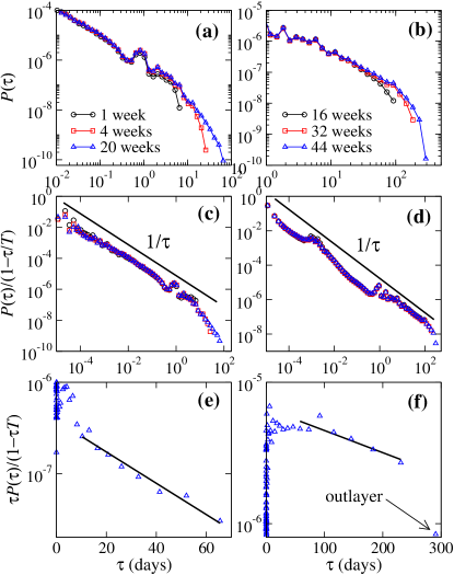
Figure 1: Distribution $P(\tau)$ of the inter-event time between two consecutive emails sent by an email user. The left and right panels represent the university and commercial datasets, respectively. For each dataset we aggregate the interevent times of all users (the distribution for single users exhibits a similar behavior Vazquez et al. (2006)) and apply a logarithmic binning to account for the fact that the number of observed events decrease with increasing $\tau$. (a) and (b) Log-log plot of $P(\tau)$ for $\tau>10^{-2}$ days, emphasizing the large $\tau$ behavior for different time window sizes $T$. (c) and (d) The same plots after removing the finite time window effects, the data collapsing into a single curve. The solid line represents the power law decay $P(\tau)\sim\tau^{-1}$. (e) and (f) Semilog plot emphasizing the exponential decay at large $\tau$, for the largest time window $T$. The solid lines are fit to an exponential decay $\tau P(\tau)\sim e^{-\tau/\tau_{\rm E}}$ resulting in $\tau_{\rm E}=25\pm 2$ days and $9\pm 1$ months for the university (e) and commercial (f) datasets, respectively. The outlayer in (f) was excluded when fitting to an exponential decay.

The dynamics of worm spreading: To investigate the impact of the observed non-Poisson activity patterns on spreading processes we study the spread of email worms among email users. For the moment we ignore the possibility that some users may delete the infected email or may have installed the worm antivirus and therefore do not participate in the spreading process, to return later at the possible impact of these events on our predictions. Therefore, the spreading process is well described by the susceptible-infected (SI) model on the email network.

The spreading dynamics is jointly determined by the email activity patterns and the topology of the corresponding email communication network Ebel et al. (2002); Eckmann et al. (2004). The email activity patterns are reflected in the infection generation times, where the generation time is defined as the time interval between the infection of the primary case (the user sending the email) and the infection of a secondary case (a different user opening the received infected email). From the perspective of the secondary case, the time when a user receives the infected email is random and the generation time is the time interval between arrival and the opening of the infected email. In most cases received emails are responded in the next email activity burst Eckmann et al. (2004); Vazquez et al. (2006), and viruses are acting when emails are read, approximately the same time when the next bunch of emails are written. Therefore the generation time can be approximated by the time interval between the arrival of a virus infected email, and the next email sent to any recipient by the secondary case. If we model the email activity pattern as a renewal process Feller (1966) with inter-event time distribution $P(\tau)$ then the generation time is the residual waiting time and is characterized by the probability density function Feller (1966)

$$g(\tau)=\frac{1}{\langle\tau\rangle}\int_{\tau}^{\infty}dxP(x)\ .$$ (2)

Next we calculate the average number of new infections $n(t)$ at time $t$ resulting from an outbreak starting from a single infected user at $t=0$. Although the email network contain cycles, it is a very sparse, thus we approximate it by a tree-like structure. Previous analytical studies have shown that this approximation captures the main features of the spreading dynamics on real networks Pastor-Satorras and Vespignani (2001); Vazquez (2006b). In this case $n(t)$ is given by Vazquez (2006b)

$$n(t)=\sum_{d=1}^{D}z_{d}g^{\star d}(t)\ ,$$ (3)

where $z_{d}$ is the average number of users $d$ email contacts away from the first infected user, $D$ is the maximum of $d$ and $g^{\star d}(t)$ is the $d$-order convolution of $g(\tau)$, $g^{\star 1}(t)=g(t)$ and $g^{\star d}(t)=\int_{0}^{t}d\tau g(\tau)g^{\star d-1}(t-\tau)$ for $d>1$, representing the probability density function of the sum of $d$ generation times. Substituting the Poisson approximation and Email data interevent time distributions into (2) and the result into (3) we obtain

$$n(t)=F(t)\exp\left(-\frac{t}{\tau_{0}}\right)\ ,$$ (4)

where $\tau_{0}=\langle\tau\rangle$ for the Poisson approximation and $\tau_{0}=\tau_{\rm E}$ for the Email data, and

$$F(t)=\left\{\begin{array}[]{ll}\frac{1}{\langle\tau\rangle}\sum_{d=1}^{D}\frac{z_{d}}{(d-1)!}\left(\frac{t}{\langle\tau\rangle}\right)^{d-1}\ ,&\mbox{Poisson approx.}\\ \sum_{d=1}^{D}z_{d}f^{\star d}(t)\ ,&\mbox{Email data}\ ,\end{array}\right.$$ (5)

where $f(t)=\int_{\tau}^{\infty}dxx^{-\alpha}e^{(tau-x)/\tau_{E}}/\langle\tau\rangle$. In the long time limit (4) is dominated by the exponential decay while $F(t)$ gives just a correction. The decay time is, however, significantly different for the Poisson approximation and the real inter-event time distribution.

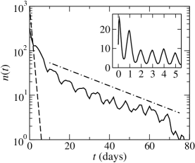
Figure 2: Average number of new infections resulting from simulations using the email history of the university dataset (solid line), using a one day interval binning. The inset shows a zoom of the initial stages of the spreading process using a one hour interval binning. The lines correspond to the exponential decay predicted by the Poisson process approximation (dashed) and the true inter-event distribution (dot-dashed).

To test these predictions we perform numerical simulations using the detailed email communication history. In this case a susceptible user receiving an infected email at time $t$ becomes infected and sends an infected email to all its email contacts at $t^{\prime}>t$, where $t^{\prime}$ is the time he/she sends an email for the first time after infection, as documented in the email data. To reduce the computational cost we focus our analysis on the smaller university dataset. The average number of new infected users resulting from the simulation exhibits daily (Fig. 2, inset) and weekly oscillations (Fig. 2, main panel), reflecting the daily and weekly periodicity of human activity patterns. More important, after ten days the oscillations are superimposed on an exponential decay, with a decay time about 21 days (see Fig. 1b). The Poisson process approximation would predict a decay time of one day, in evident disagreement with the simulations (Fig. 2). In contrast, using the correct inter-event time distribution for the university dataset we predict a decay time of $25\pm 2$ days, in good agreement with the numerical simulations (Fig. 2).

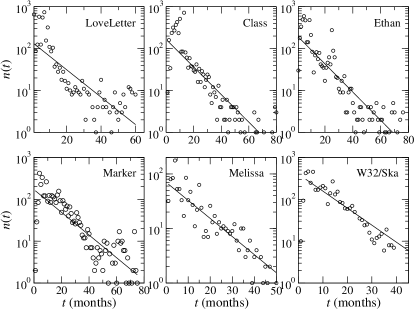
Figure 3: Number new infections reported for six worm outbreaks, according to Virus Bulletin (www.virusbtn.com). The lines are fit to an exponential decay resulting in the decay times (measured in months): LoveLetter ($13\pm 2$), Ethan ($12\pm 1$), Marker ($14\pm 2$), Class ($12\pm 1$), Melissa ($13\pm 1$), W32/Ska ($11\pm 1$).

The analysis of the university dataset allows us to demonstrate the connection between the long $\tau$ behavior of the inter-event time distribution $P(\tau)$ and the long time decay of the prevalence $n(t)$. Our main finding is that the prevalence decay time is given by the characteristic decay time of the inter-event time distribution. More important, we show that the Poisson process approximation clearly underestimates the decay time. For Poisson processes the two time scales, the average interevent time and the characteristic time of the exponential decay coincide, being both of the order of one to at most a few days. Using measurements on the commercial dataset, containing a larger number of individuals and covering a wider spectrum of email users, we can extrapolate these conclusions to predict the behavior of real viruses. Given the value of $\tau_{\rm E}$ for the commercial dataset we predict that the email worm prevalence should decay exponentially with time, with a decay time about nine months. The prevalence tables reported by the Virus Bulletin web site (http://www.virusbtn.com) indicate that worm outbreaks persist for several months, following an exponential decay with a decay time around twelve months (Fig. 3). Our nine month prediction is thus much closer to the observed value than the $\langle\tau\rangle\approx 1\div 4$ day prediction based on the Poisson approximation. The fact that our prediction underestimates the actual decay time by about three months is probably rooted in the fact that the commercial dataset, despite its coverage of an impressive 1.7 million users, still captures only a small segment (approximately 0.1%) of all Internet users.

As we discussed above, some other factors potentially affecting the spreading of email worms were not considered in our analysis. First, some users may delete the infected emails or may have installed the worm antivirus. Since these users do not participate in the spreading process they are eliminated from the average number users $z_{d}$ that are found $d$ email contacts away from the first infected user. While this would affect the initial spread characterized by $F(t)$ (5), the exponential decay in (4) and the decay time $\tau_{0}=\tau_{\rm E}$ will not be altered. Second, some email viruses do not use the self-broadcasting mechanism of email worms. For example, file viruses require the email user to attach the infected file into a sent email in order to be transmitted. In turn, only some email contacts will receive the infected file. Once again, this affects $z_{d}$ but not the email activity patterns. Therefore, the prevalence of email viruses in general should decay exponentially in time with a decay time $\tau_{0}$ determined by the decay time of the inter-event time distribution $\tau_{\rm E}$. Third, new virus strains regularly emerge following small modifications of earlier viruses. Within this work new virus strains are modeled as new outbreaks. An alternative approach is to analyze all strains together, modeling the emergence of new strains as a process of reinfection. In this second approach the dynamics is better described by the susceptible-infected-susceptible (SIS) model Pastor-Satorras and Vespignani (2001). Earlier work has shown that if reinfections are allowed in networks with a power law degree distribution, long prevalence decay times may emerge, which increase with increasing the network size Pastor-Satorras and Vespignani (2001). The data shown in Fig. 3 represent, however, the spread of a single virus strain, which is better captured by the SI model. For the SI model, however, for a Poisson activity pattern we should get a rapid decay in prevalence, indicating that the empirically observed long decay times cannot be attributed to this reinfection-based mechanism.

A series of recent measurements indicate that power law inter-event time distributions are not a unique feature of email communications, but emerge in a wide range of human activity patterns, describing the timing of financial transactions Plerou et al. (2000); Masoliver et al. (20003), response time of internauts Johansen (2001), online games Henderson and Nhatti (2001), login times into email servers Chatterjee and printing processes Harder and Paczuski (2006). Together they raise the possibility that non-Poisson contact timing are a common feature of human dynamics and thus could impact other spreading processes as well. Indeed, measurements indicate that the patterns of visitation of public places, like libraries Vazquez et al. (2006), or the long range travel patterns of humans, involving car and air travel, is also driven by fat tailed inter-event times Brockmann et al. (2006). Such travel patterns play a key role in the spread of biological viruses, such as influenza or SARS Colizza et al. (2006). Taken together, these results indicate that the anomalous decay time predicted and observed for email viruses may in fact apply more widely, potentially impacting the spread of biological viruses as well.

Acknowledgements: We wish to thank Deok-Sun Lee for useful comments on the manuscript. This work was supported by a grant from the James McDonell Foundation and NSF, by a Yahoo Faculty Research Grant and grant ASTOR NKFP 2/004/05, and the Mobile Innovation Center, Hungary.

References

- Pastor-Satorras and Vespignani (2001) R. Pastor-Satorras and A. Vespignani, Phys. Rev. Lett. 86, 3200 (2001).
- Anderson and May (1991) R. M. Anderson and R. M. May, Infectious diseases of humans (Oxford Univ. Press, New York, 1991).
- Meyers et al. (2005) L. A. Meyers, B. Pourbohloul, M. E. J. Newman, D. M. Skowronski, and R. C. Brunham, J Theor. Biol. 232, 71 (2005).
- Moreno et al. (2002) Y. Moreno, R. Pastor-Satorras, and A. Vespignani, Eur. Phys. J. B 26, 521 (2002).
- Barthélemy et al. (2004) M. Barthélemy, A. Barrat, R. Pastor-Satorras, and A. Vespignani, Phys. Rev. Lett. 92, 178701 (2004).
- Boccaletti et al. (2006) S. Boccaletti, V. Latora, Y. Moreno, M. Chavez, and D.-U. Hwang, Phys. Rep. 424, 175 (2006).
- Moreno et al. (2004) Y. Moreno, M. Nevokee, and A. F. Pacheco, Phys. Rev. E 69, 066130 (2004).
- (8) M. Nekovee, Y. Moreno, G. Bianconi, and M. Marsili, arXiv:physics/0508008.
- Pastor-Satorras and Vespignani (2004) R. Pastor-Satorras and A. Vespignani, Evolution and structure of the Internet: A Statistical Physics approach (Cambridge University Press, Cambridge, 2004).
- Eckmann et al. (2004) J.-P. Eckmann, E. Moses, and D. Sergi, Proc. Natl. Acad. Sci. USA 101, 14333 (2004).
- Johansen (2004) A. Johansen, Physica A 338, 286 (2004).
- Barabási (2005) A.-L. Barabási, Nature 435, 207 (2005).
- Vazquez et al. (2006) A. Vazquez, J. G. Oliveira, Z. Dezső, K.-I. Goh, I. Kondor, and A.-L. Barabási, Phys. Rev. E 73, 036127 (2005); J. G. Oliveira and A.-L. Barabási, Nature 437, 1251 (2006).
- Vazquez (2006a) A. Vazquez, Physica A 373, 747 (2007).
- Vazquez (2005) A. Vazquez, Phys. Rev. Lett. 95, 248701 (2005).
- Feller (1966) W. Feller, An introduction to probability theory and its applications (Wiley, New York, 1966), vol. II.
- Ebel et al. (2002) H. Ebel, L.-I. Mielsch, and S. Bornholdt, Phys. Rev. E 66, 035103 (2002).
- Vazquez (2006b) A. Vazquez, Phys. Rev. Lett. 96, 038702 (2006b).
- Plerou et al. (2000) V. Plerou, P. Gopikirshnan, L. Amaral, X. Gabaix, and H. Stanley, Phys. Rev. E 62, R3023 (2000).
- Masoliver et al. (20003) J. Masoliver, M. Montero, and G. Weiss, Phys. Rev. E 67, 021112 (20003).
- Johansen (2001) A. Johansen, Physica A 296, 539 (2001).
- Henderson and Nhatti (2001) T. Henderson and S. Nhatti, in Proc. ACM Multimedia 2001, Ottawa, Canada (2001), pp. 212–220.
- (23) A. Chatterjee, arXive:cond-mat/0307533.
- Harder and Paczuski (2006) R. Harder and M. Paczuski, Physica A 361, 329 (2006).
- Brockmann et al. (2006) D. Brockmann, L. Hufnagel, and T. Geisel, Nature 439, 462 (2006).
- Colizza et al. (2006) V. Colizza, A. Barrat, M. Barthelemy, and A. Vespignani, Proc. Natl. Acad. Sci. USA 103, 2015 (2006).