Experimental study of laser detected magnetic resonance based on atomic alignment

Abstract

We present an experimental study of the spectra produced by optical/radio-frequency double resonance in which resonant linearly polarized laser light is used in the optical pumping and detection processes. We show that the experimental spectra obtained for cesium are in excellent agreement with a very general theoretical model developed in our group Weis et al. (2006) and we investigate the limitations of this model. Finally, the results are discussed in view of their use in the study of relaxation processes in aligned alkali vapors.

I Introduction

Optically pumped alkali vapor magnetometers (OPM) using circularly polarized light are widely used in many applications. One of the most common realizations is the so-called $M_{x}$ magnetometer Bloom (1962), where circularly polarized light is used to create a macroscopic spin polarization (orientation) in a vapor of alkali atoms at an angle of $45\deg$ with respect to the static magnetic field $\boldsymbol{B}_{0}$ under investigation. A small additional magnetic field $\boldsymbol{B}_{1}(t)$, hereafter referred to as radio-frequency or rf field, oscillating at a frequency close to the Larmor frequency, induces oscillations of sublevel coherences in the sample. These coherent oscillations lead to a modulation of the transmitted light power at the rf frequency, which shows a resonant behavior when the rf frequency is close to the Larmor frequency. Either the resonant amplitude change or the resonant phase change can be used to infer the magnetic field modulus. Discharge lamps are commonly used light sources for alkali OPMs. Such lamps emit a broad spectrum and can be used for optical pumping only when a single fine structure component, typically the $\mathrm{D}_{1}$-line for alkalis, is isolated by means of an appropriate filter Happer (1972).

Pumping with circularly polarized light builds up a vector polarization (orientation), while pumping with linearly polarized light leads to the creation of a tensor polarization (alignment) in the atomic ground state, provided that it has an angular momentum larger than $1/2$. The ground state of alkali atoms has an electronic angular momentum $J=1/2$, which can not be aligned. However, the hyperfine interaction with the nuclear spin $I$ splits the ground state into two hyperfine levels with total angular momenta $F_{\pm}=|I\pm 1/2|$, which can be aligned provided $F\geq 1$. An alignment can therefore be prepared, or detected, if the light source has a sufficient spectral resolution to excite a single hyperfine transition. In general, this is not the case for the Doppler and pressure–broadened spectrum of discharge lamps.

The first detection of an optically induced alignment was reported in ${}^{4}\!\mathrm{He}$Bell and Bloom (1961). Later, both DC signals and signals oscillating at the fundamental and at the second harmonic of the alignment precession frequency have been observed in ${}^{87}\!\mathrm{Rb}$ via birefringence measurements Mathur et al. (1970) using a double beam technique. In Aleksandrov and Balabas (1990) the authors observed the alignment in a lamp-pumped ${}^{87}\!\mathrm{Rb}$ vapor by analyzing the induced linear birefringence of the vapor while using the same light beam for pumping and probing the atoms. The creation and detection of atomic alignment with radiation from a discharge lamp becomes possible when using an isotope filtering technique Aleksandrov and Balabas (1990); Mathur et al. (1970) for isolating specific hyperfine components. However, that technique is restricted to Rb and can neither be applied to Na nor to K, where the lamp emission spectrum leaves the hyperfine structure unresolved, nor to Cs for which no isotope filters are available.

Due to their narrow spectral widths (several MHz compared to the Doppler broadening of several hundred MHz), tunable lasers provide a way to selectively drive an isolated optical hyperfine transition, a very effective way to create an alignment with linearly polarized light. Narrow-band tunable laser sources are therefore an interesting alternative to spectral lamps for magnetometric applications. Their use in $M_{x}$ magnetometers has been demonstrated Aleksandrov et al. (1995) and it could be shown that laser-based alkali magnetometers yield a superior magnetometric performance compared to lamp pumped devices Aleksandrov et al. (1995); Groeger et al. (2005). A discussion of laser pumping with circularly and linearly polarized light in ${}^{4}\!\mathrm{He}$ can be found in Gilles et al. (1992, 2001). Those authors investigated several magnetometry techniques using both orientation and alignment signals and observed magnetic resonances by applying either rf fields, light intensity modulation, polarization modulation, or laser frequency modulation. A variant of the latter technique in which the polarization of the transmitted light was measured, rather than its intensity, was realized with ${}^{87}\!\mathrm{Rb}$ by Budker et al. (2000, 2002).

In a recent publication Weis et al. (2006), our group presented a theoretical study of the spectra produced by optical/radio-frequency double resonance devices in which resonant linearly polarized light is used in the optical pumping process. That study led to very general algebraic results, valid for atomic states with arbitrary angular momenta, for arbitrary rf intensities, and for arbitrary geometries, valid however only for low laser light power. Therefore, our goal was to investigate experimentally the domain of validity of this theoretical model.

In this work, we present an experimental investigation of the magnetic resonance spectra produced in a cesium vapor in which an alignment is created and detected by a single linearly polarized laser beam. We show that the experimental spectra obtained for cesium are in excellent agreement with the theoretical model presented in Weis et al. (2006) and we investigate the limitations of this model. In contrast to prior work reported in Mathur et al. (1970); Aleksandrov and Balabas (1990); Gilles et al. (1992) we detect the signal at both the first and second-harmonic of the applied rf field. This offers the possibility of detecting the alignment in low magnetic fields where the quadratic Zeeman splitting is negligible. The technique reported in Aleksandrov and Balabas (1990) is insensitive to alignment in small fields since the signals at the first harmonic cancel each other in the low field limit.

II Experiments

II.1 Principle

Figure 1: Geometry of double resonance spectroscopy involving linearly polarized light. The oscillating field $\boldsymbol{B}_{1}$ rotates in a plane perpendicular to the static field $\boldsymbol{B}_{0}$. The linear polarization vector $\boldsymbol{\epsilon}$ makes an angle $\gamma$ with the static field $\boldsymbol{B}_{0}$, and the phase of $\boldsymbol{B}_{1}$ is characterized by $\alpha$.

The experimental geometry, shown in Fig. 1, is identical to the one described in Weis et al. (2006). A linearly polarized laser beam, resonant with a given hyperfine transition, creates an atomic alignment in a room temperature vapor of cesium atoms by optical pumping. This alignment is driven coherently by simultaneous interactions with the optical field, a static magnetic field $\boldsymbol{B}_{0}$, a much weaker rotating magnetic field $\boldsymbol{B}_{1}$, and is affected by relaxation processes. The rf field $\boldsymbol{B}_{1}$ rotates in a plane perpendicular to $\boldsymbol{B}_{0}$ at frequency $\omega$. The steady state dynamics are probed by monitoring the transmitted light power.

The precession of the alignment driven by the rf field leads to modulations of the transmitted power at both the fundamental and the second harmonic of the rf frequency $\omega$. Lock-in detection is used to record spectra of the first and second harmonic signals and the results are compared with the theoretical predictions of Weis et al. (2006). We investigated the effects of the experimental parameters on the spectral line shapes of the in-phase and quadrature components of both signals. In particular, we studied the dependence of the signals on the angle $\gamma$ between the linear polarization vector and the static field, the dependence on rf power, and the dependence on light power.

II.2 Experimental setup

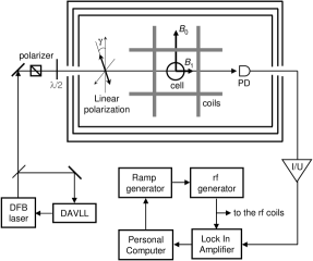
Figure 2: Sketch of the experimental setup. A paraffin-coated glass cell containing Cs vapor was placed inside a three-layer mumetal shield. The shield contained Helmholtz coils to produce the static magnetic field $\boldsymbol{B}_{0}$, and radio-frequency coils to produce the rotating magnetic field $\boldsymbol{B}_{1}$. The DFB diode laser was stabilized to the $F_{g}=4\rightarrow F_{e}=3$ transition of the Cs $\mathrm{D}_{1}$ line by means of a dichroic atomic vapor laser lock (DAVLL). A linear polarizer followed by a half-wave plate ($\lambda/2$) were used to prepare linearly polarized light at an angle $\gamma$ with respect to $\boldsymbol{B}_{0}$. The transmitted light power after the cell was monitored by a nonmagnetic photodiode (PD) whose signal was amplified by a low-noise transimpedance amplifier and analyzed by a lock-in amplifier. The function generator driving the rf field also served as reference for the lock-in amplifier. The resonance spectra were recorded by a personal computer which controlled the rf frequency scan.

The measurements were done using a room temperature cesium vapor in vacuum confined within a paraffin-coated spherical glass cell (28 mm diameter). The experimental setup is shown in Fig. 2. The cesium vapor cell was isolated from ambient magnetic fields by a three-layer mumetal shield. Inside the shield, a pair of Helmholtz coils produced a static magnetic field $\boldsymbol{B}_{0}$ of about $3\>\mu\mathrm{T}$ perpendicular to the light propagation direction. Additional orthogonal pairs of Helmholtz coils (only one pair is shown in Fig. 2) were used to compensate residual transverse fields and gradients. An rf magnetic field $\boldsymbol{B}_{1}$, rotating at approximately 10 kHz in the plane perpendicular to the static magnetic field, was created by a set of two pairs of Helmholtz coils, wound on the same supports as the static field coils. The laser beam used to pump and probe the atomic vapor was generated by a DFB diode laser ($\approx 894\>\mbox{nm}$) stabilized to the $6S_{1/2},F_{g}\!=\!4\!\rightarrow\!6P_{1/2},F_{e}\!=\!3$ hyperfine component by means of a dichroic atomic vapor laser lock (DAVLL) Corwin et al. (1998). A linear polarizer followed by a half-wave plate prepared linearly polarized light of adjustable orientation $\gamma$ with respect to $\boldsymbol{B}_{0}$. After the half-wave plate, the remaining degree of circular polarization was smaller than 1%. The light power transmitted through the cell was detected by a nonmagnetic photodiode, whose photocurrent was amplified by a low-noise transimpedance amplifier. The resulting signal was analyzed by a lock-in amplifier tuned either to the first or second harmonic of the rf frequency. Magnetic resonance spectra were recorded by sweeping the rf frequency and simultaneously recording the in-phase and quadrature signals from the lock-in amplifier. The first harmonic and second harmonic signals were recorded in sequential scans under identical conditions.

III DRAM theoretical model

The double resonance alignment magnetometer model (DRAM model) developed in Weis et al. (2006) provides algebraic expressions for the expected resonance signals. In that model, the line shapes are calculated following a three-step approach: creation of alignment by optical pumping, magnetic resonance, and detection of the oscillating steady state alignment. In practice, the three steps occur simultaneously and the approach is valid only if steady state conditions are reached for the first two steps. As explained in Weis et al. (2006), the approach is thus valid only if the optical pumping rate is negligible compared to the relaxation rates, i.e., for low light powers. The model calculates the evolution of the alignment multipole moments $m_{2,q}$ via a density matrix approach, where the moments $m_{2,q}$ are defined with respect to a quantization axis aligned with $\boldsymbol{B}_{0}$ and relax with rates $\Gamma_{\kern-1.60997pt|q|}$. The third step probes the state of the $m_{2,q}$ and results in detectable signals.

Only the most relevant equations needed for the analysis of the presented measurements are reproduced here. The magnetometer signals which are modulated at the rf frequency $\omega$ and at its second harmonic $2\omega$, can be written as

$$S_{\omega}(t) \!\!\!=\phantom{{}_{2}}\mathcal{A}_{0}\,h_{\omega}(\gamma)\left[\right. \!\!\!\phantom{-}D_{\omega}\,\cos\left(\omega t-\alpha\right)$$ (1a)

$$\!\!\!\left.-A_{\omega}\,\sin\left(\omega t-\alpha\right)\right]\,,$$

$$S_{2\omega}(t) \!\!\!=\mathcal{A}_{0}\,h_{2\omega}(\gamma)\left[\right. \!\!\!-A_{2\omega}\,\cos\left(2\omega t-2\alpha\right)$$ (1b)

$$\!\!\!\left.-D_{2\omega}\,\sin\left(2\omega t-2\alpha\right)\right]\,,\quad\phantom{,}$$

where $\mathcal{A}_{0}$ is the alignment produced by the linearly polarized laser light in the first step of the model. The phase of the rf field with respect to $\boldsymbol{k}\times\boldsymbol{B}_{0}$ is $\alpha$ (cf. Fig. 1). The angular dependencies of the first and second harmonic signals are given by

$$h_{\omega}(\gamma) = \frac{3}{16}\left(2\sin 2\gamma+3\sin 4\gamma\right)\,,$$ (2a)

$$h_{2\omega}(\gamma) = \frac{3}{32}(1-4\cos 2\gamma+3\cos 4\gamma)\,,$$ (2b)

where we have chosen an alternative representation of the expressions given in Weis et al. (2006). The first and second harmonic signals have both absorptive, $A_{\omega}$, $A_{2\omega}$, and dispersive, $D_{\omega}$, $D_{2\omega}$, components in their line shapes, given by

$$D_{\omega} = \frac{\delta\,\Gamma_{\kern-1.60997pt0}\omega_{1}(\Gamma_{\kern-1.60997pt2}^{2}+4\delta^{2}-2\omega_{1}^{2})}{Z}\,,$$ (3a)

$$A_{\omega} = \frac{\phantom{\delta\,}\Gamma_{\kern-1.60997pt0}\omega_{1}\left[(\Gamma_{\kern-1.60997pt2}^{2}+4\delta^{2})\Gamma_{\kern-1.60997pt1}+\Gamma_{\kern-1.60997pt2}\omega_{1}^{2}\right]}{Z}\,,$$ (3b)

$$D_{2\omega} = \frac{\delta\,\Gamma_{\kern-1.60997pt0}\omega_{1}^{2}(2\Gamma_{\kern-1.60997pt1}+\Gamma_{\kern-1.60997pt2})}{Z}\,,$$ (3c)

$$A_{2\omega} = \frac{\phantom{\delta\,}\Gamma_{\kern-1.60997pt0}\omega_{1}^{2}(\Gamma_{\kern-1.60997pt1}\Gamma_{\kern-1.60997pt2}-2\delta^{2}+\omega_{1}^{2})}{Z}\,,$$ (3d)

with

$$Z = \Gamma_{\kern-1.60997pt0}\left(\Gamma_{\kern-1.60997pt1}^{2}+\delta^{2}\right)\left(\Gamma_{\kern-1.60997pt2}^{2}+4\delta^{2}\right)$$ (4)

$${}+\left[\Gamma_{\kern-1.60997pt1}\Gamma_{\kern-1.60997pt2}\left(2\Gamma_{\kern-1.60997pt0}+3\Gamma_{\kern-1.60997pt2}\right)-4\delta^{2}\left(\Gamma_{\kern-1.60997pt0}-3\Gamma_{\kern-1.60997pt1}\right)\right]\omega_{1}^{2}$$

$${}+\left(\Gamma_{\kern-1.60997pt0}+3\Gamma_{\kern-1.60997pt2}\right)\omega_{1}^{4}\,.$$

In Eqs. (3) and (4), $\omega_{1}=\gamma_{F}B_{1}$ is the Rabi frequency of the rf field where $\gamma_{F}$ is the Landé g-factor of the ground state hyperfine level $F$. The detuning, $\delta=\omega-\omega_{0}$, is the difference between the radio frequency $\omega$ and the Larmor frequency $\omega_{0}=\gamma_{F}B_{0}$.

IV Analysis of the resonance signals

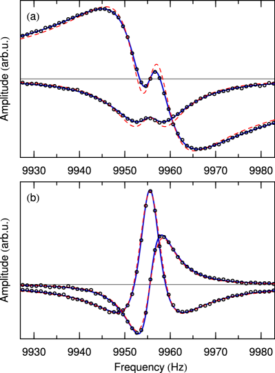
Figure 3: (Color online) Measurements (circles) of the in-phase and quadrature magnetic resonance signals detected as amplitude modulations of the transmitted light power. (a) First harmonic signals. (b) Second harmonic signals. The statistical uncertainty on each data point is smaller than the symbol size. The solid lines (blue) are fits of the theoretical line shapes given by Eqs. (3) with three independent relaxation rates. The dashed lines (red) are fits of the theoretical line shapes given by Eqs. (3) with only one independent relaxation rate $\Gamma\equiv\Gamma_{\kern-1.60997pt0}=\Gamma_{\kern-1.60997pt1}=\Gamma_{\kern-1.60997pt2}$. The details of the experimental conditions and fit results are in the text.

Typical measurements of the in-phase and quadrature spectra of the first and second harmonic signals are shown in Fig. 3. Each pair of curves was recorded in a single scan, with a lock-in time constant of 10 ms, and a sweep rate of 1 Hz/s. Note that the same scan parameters were used for all other magnetic resonance spectra presented in this paper. The data of Fig. 3 were obtained with a laser light power of $0.1\>\mu\mathrm{W}$ (approximate Gaussian profile, $1/e^{2}$ full width of 3.7 mm horizontally and 3.2 mm vertically), an rf field Rabi frequency of $\omega_{1}/(2\pi)=3.8~{}\mathrm{Hz}$, and an angle between the linear polarization vector and the static magnetic field of $\gamma=75\deg$.

In practice, lock-in detection of the signals given by Eqs. (1) with respect to the rf frequency $\omega$ adds a phase $\phi_{l}$, selectable in the lock-in amplifier, and a small pick-up signal $p_{(1,2)(A,D)}$ (smaller than 1% of the signal at maximum) to each of the line shapes in Eqs. (3). The pick-up is due to direct inductive coupling between the rf field coils and the photodiode readout wires: as expected, it varied with rf power but not with $\delta$. Due to $\phi_{l}$, the in-phase and quadrature spectra are, in general, a mixture of dispersive and absorptive line shapes. Indeed, after demodulation of the signal given by Eq. (1a), we obtain the following expressions which were used to fit the in-phase and quadrature spectra

$$I_{\omega}(\delta)\! \!=g_{\omega}\mathcal{A}_{0}h_{\omega}(\gamma) \kern-4.30554pt\left[\phantom{+}(D_{\omega}+p_{1D})\cos{(\alpha\!+\!\phi_{l})}\right.$$ (5a)

$$\kern-4.30554pt\left.\,+(A_{\omega}+p_{1A})\sin{(\alpha\!+\!\phi_{l})}\right]$$

$$Q_{\omega}(\delta)\! \!=g_{\omega}\mathcal{A}_{0}h_{\omega}(\gamma) \kern-4.30554pt\left[\phantom{+}(A_{\omega}+p_{1A})\cos{(\alpha\!+\!\phi_{l})}\right.$$ (5b)

$$\kern-4.30554pt\left.\,-(D_{\omega}+p_{1D})\sin{(\alpha\!+\!\phi_{l})}\right]$$

A similar mix of $A_{2\omega}$ and $D_{2\omega}$ was used for the second harmonic signal given by Eq. (1b). Due to frequency dependent phase shifts in the signal treatment electronics, both the effective $\phi_{l}$ and the pickup terms ($p_{1A}$, $p_{1D}$, $p_{2A}$, $p_{2D}$) were different for the $\omega$ and $2\omega$ signals. Global detection factors, $g_{\omega}$ and $g_{2\omega}$, were also required to model amplifier dependent gains and light power dependent effects other than the creation of $\mathcal{A}_{0}$. In total, nine free parameters were needed to fit an in-phase plus quadrature signal pair, while only thirteen were needed to fit all four signals simultaneously since the physics parameters ($\omega_{0}$, $\omega_{1}$, $\Gamma_{\kern-1.60997pt0}$, $\Gamma_{\kern-1.60997pt1}$, and $\Gamma_{\kern-1.60997pt2}$) were the same for both harmonics. All results for those parameters reported in this paper were taken, when possible, from simultaneous four-spectra fits.

Leaving $\Delta\alpha$$=(\alpha+\phi_{l})$ free during the fits to the data had the advantage of simplifying the experimental procedure and gave access to the phase information, which was used to adjust the direction of the static magnetic field. Indeed, for the measurements testing the angular dependence of the resonance signals (see §V), it is important that the static magnetic field is exactly perpendicular to the laser beam wave vector, as shown in Fig. 1. This is the case when the phase mismatch $\Delta\alpha$ obtained from the fitting procedure is independent of the angle $\gamma$ between the polarization and the static magnetic field.

In order to check the validity of the model developed in Weis et al. (2006), the theoretical line shapes were fitted to the experimental data: the resulting curves are plotted with the experimental data in Fig. 3. The solid lines were obtained using Eqs. (3) with three independent relaxation rates: $\Gamma_{\kern-1.60997pt0}$ for the relaxation of populations, $\Gamma_{\kern-1.60997pt1}$ for the relaxation of $\Delta M=\pm 1$ coherences, and $\Gamma_{\kern-1.60997pt2}$ for the relaxation of $\Delta M=\pm 2$ coherences. As a result of the fit we obtained $\Gamma_{\kern-1.60997pt0}/(2\pi)=1.64(2)\>\mathrm{Hz}$, $\Gamma_{\kern-1.60997pt1}/(2\pi)=2.93(2)\>\mathrm{Hz}$ and $\Gamma_{\kern-1.60997pt2}/(2\pi)=3.08(2)\>\mathrm{Hz}$.

Note that the longitudinal relaxation rate $\Gamma_{\kern-1.60997pt0}$ is quite different from the transverse relaxation rates $\Gamma_{\kern-1.60997pt1,2}$, demonstrating that it is not possible to obtain a good fit with a simpler model with only one single relaxation rate $\Gamma\equiv\Gamma_{\kern-1.60997pt0}=\Gamma_{\kern-1.60997pt1}=\Gamma_{\kern-1.60997pt2}$. In that case the line shape functions have a relatively simple algebraic form which is given in Weis et al. (2006). A fit of the simplified model is shown as dashed curves in Fig. 3 and yielded a $\chi^{2}$-minimizing value of $\Gamma/(2\pi)=2.80(4)\>\mathrm{Hz}$. As expected, the fit quality is poor compared to the model with three independent relaxation rates.

Since the values of the transverse rates $\Gamma_{\kern-1.60997pt1}$ and $\Gamma_{\kern-1.60997pt2}$ differ by less than 5%, it is possible to use a model with two relaxation rates, $\Gamma_{\kern-1.60997ptL}\equiv\Gamma_{\kern-1.60997pt0}$ and $\Gamma_{\kern-1.60997ptT}\equiv\Gamma_{\kern-1.60997pt1}=\Gamma_{\kern-1.60997pt2}$, without significantly degrading the fit quality. Curves representing a fit with only two independent relaxation rates ($\Gamma_{\kern-1.60997ptL},\Gamma_{\kern-1.60997ptT}$) are not shown in Fig. 3 because they are indistinguishable from the solid lines obtained with three independent relaxation rates. However, we found that the ratio of $\Gamma_{\kern-1.60997pt1}$ to $\Gamma_{\kern-1.60997pt2}$ depends on the angle $\gamma$, and that it changes with laser power. Therefore, the model with three relaxation rates will be used for the rest of this work.

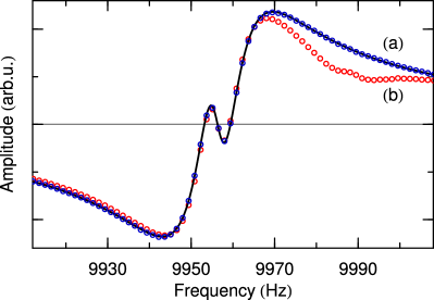
Figure 4: (Color online) Dispersive component of the magnetic resonance signal oscillating at frequency $\omega$ measured under the following conditions: the angle between the linear polarization vector and the static field was $\gamma=25\deg$, the laser light power was $0.1\>\mu\mathrm{W}$, and the rf field Rabi frequency was $\omega_{1}/(2\pi)=4.8~{}\mathrm{Hz}$. Graph (a) (blue) was measured with a rotating rf field and graph (b) (red) with an oscillating rf field. The solid line is a fit of the theoretical line shape to the curve obtained with the rf rotating field. The slight difference in linewidth suggests that the Rabi frequency in the two measurements was not perfectly equal although we increased the amplitude of the oscillating rf field by a factor 2.

Note that the use of a rotating rf field is crucial for the quality of the fits. Magnetic resonance experiments, and in particular optically pumped magnetometers, usually use a linearly polarized rf field. The implementation of such a field is technically less demanding and its use is justified, in high-Q oscillators with a single resonance frequency, by the rotating wave approximation by virtue of which the precessing spins interact only with the circularly polarized component of the rf field that co-rotates with the spins.

When using an oscillating rf field one obtains the spectrum (b) shown in Fig. 4, while the use of a rotating rf field yields the spectrum (a). Spectrum (b) shows a second weak resonance located approximately 33 Hz above the main resonance. That difference frequency corresponds to the difference of the Larmor frequencies of the $F_{g}=4$ and $F_{g}=3$ ground state hyperfine levels due to the nuclear magnetic moment term in the expression for the gyromagnetic ratio $g_{F}$.

The structure can be explained as follows: Optical pumping aligns both the $F_{g}=3$ and the $F_{g}=4$ ground states and magnetic resonance transitions can be driven within these two states. The resonance in the $F_{g}=3$ state is not detected directly since the laser frequency is adjusted to the $F_{g}=4\rightarrow F_{e}=3$ transition. However, spin exchange collisions can transfer the alignment from the $F_{g}=3$ to the $F_{g}=4$ state where it can be detected. In principle, this opens a way for the experimental study of alignment transfer collisions. In our experiment, the use of a rotating rf field allowed us to record spectra without contamination from the $F_{g}=3$ state. This is due to the $g_{F}$-factors of both states having opposite signs, so that they precess in opposite directions, and the rotating field thus co-rotates with one species only, i.e., the $F_{g}=4$ atoms.

V Angular dependence

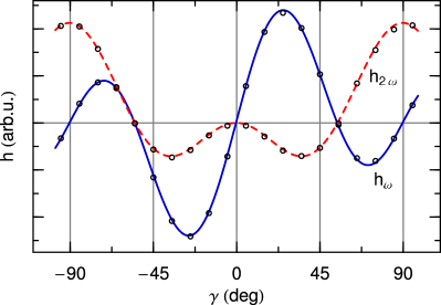
Figure 5: (Color online) Angular dependence of the amplitude of the first (blue, solid line) and second (red, dashed line) harmonic signals on the angle $\gamma$ between the light polarization $\boldsymbol{\epsilon}$ and the magnetic offset field $\boldsymbol{B}_{0}$. Each experimental data point is the result of a measurement and fit of the magnetic resonance spectra as explained in §IV. The measurements were made using a light power of $0.07\>\mu\mathrm{W}$ and a rf field Rabi frequency of $2.4~{}\mathrm{Hz}$. The lines were found by fitting the $h_{\omega}$ and $h_{2\omega}$ functions given by Eqs. (2) to the experimental data.

Our theoretical DRAM model gives algebraic results which are valid for arbitrary geometries. To check the angular dependencies predicted by the model we measured and fit the magnetic resonance spectra for different values of $\gamma$, the angle between the linear polarization vector and the static magnetic field. All fit qualities were comparable to that of Fig. 3. From the fits, the amplitudes of the first and second harmonic signals were determined and the results are plotted as circles in Fig. 5. The solid and dashed lines represent the theoretical angular dependencies $h_{\omega}$ and $h_{2\omega}$ given by Eqs. (2). The agreement is very good.

A crucial point for these measurements was the quality of the linear polarization, a parameter found to be particularly important for small angles. Indeed, both the first and second harmonic signals should disappear when $\gamma$ is very small, and therefore any small contamination of circular polarization produces a visible parasitic resonance signal. For that reason we used a high quality Glan-prism to produce linear polarization with a degree of circular polarization (DOCP) on the order of 0.1%. However, the imperfection of the half-wave plate used to rotate the polarization vector somewhat degraded the quality of the polarization. In spite of that, a DOCP of less than 1% could be maintained over the range of angles $\gamma$ investigated, which proved to be sufficient for the measurements. Careful inspection of the angular dependence of the second harmonic signal ($h_{2\omega}$ in Fig. 5) reveals that all experimental points near $\gamma=0$ lie below the theoretical curve. This is a typical effect from circular polarization contamination, as verified by intentionally increasing the DOCP, e.g., by using a polarizer of poorer quality.

VI Dependence on the rf power

Figure 6: Resonance spectra measured with an angle $\gamma=75\deg$ and for different Rabi frequencies of the rf field: (a) $\omega_{1}/(2\pi)=0.95~{}\mathrm{Hz}$, (b) $\omega_{1}/(2\pi)=2.4~{}\mathrm{Hz}$, (c) $\omega_{1}/(2\pi)=4.8~{}\mathrm{Hz}$. The left column shows in-phase and quadrature components of the first harmonic signal, and the right column shows in-phase and quadrature components of the second harmonic signal. For these measurements, the light power was $0.1\>\mu\mathrm{W}$.

The DRAM theoretical model gives algebraic results which are valid for arbitrary rf intensities. Its predictions were checked by measuring and fitting magnetic resonance spectra for selected values of the Rabi frequency of the rf field. Three sets of illustrative spectra are presented in Fig. 6 together with the respective fits. The resonance curves were measured at a fixed angle $\gamma=75\deg$ and for $\omega_{1}/(2\pi)=0.95~{}\mathrm{Hz}$, $2.4~{}\mathrm{Hz}$, and $4.8~{}\mathrm{Hz}$. The quality of the fits does not depend on the rf intensity. Moreover, all twelve curves were fitted with the same unique set of physics parameters. In the presented data, the common values for relaxation rates are $\Gamma_{\kern-1.60997pt0}/(2\pi)=1.64(1)\>\mathrm{Hz}$, $\Gamma_{\kern-1.60997pt1}/(2\pi)=2.98(1)\>\mathrm{Hz}$ and $\Gamma_{\kern-1.60997pt2}/(2\pi)=3.05(1)\>\mathrm{Hz}$. This shows that the evolution of the resonance spectra with rf power is well described by the DRAM theoretical model.

In particular, note the appearance of the narrow spectral feature in the first harmonic signal as the rf power is increased. This feature emerges as predicted by the DRAM theoretical model for $\omega_{1}>\Gamma_{\kern-1.60997pt2}/\sqrt{2}$. As discussed in Weis et al. (2006), it can be explained as a product of the creation of a $\Delta M=2$ coherence by a second order interaction with the rf field, followed by the evolution of that coherence in the offset field, and back-transfer to a $\Delta M=1$ coherence by an additional interaction with the rf field, which can then be detected at the first harmonic frequency $\omega$. In our measurement, $\Gamma_{\kern-1.60997pt2}/\sqrt{2}=2\pi\times 2.16\>\mathrm{s}^{-1}$ and we indeed observe this narrow spectral feature when $\omega_{1}/(2\pi)$ becomes larger than $2.16\>\mathrm{Hz}$. Note that this feature allows an easy calibration of the rf voltage applied to the coils in terms of the resulting Rabi frequency $\omega_{1}$.

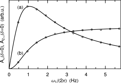
Figure 7: Saturation of the resonant absorptive signals $A_{\omega}$ and $A_{2\omega}$ as a function of the Rabi frequency $\omega_{1}/(2\pi)$ of the rf field. (a) On-resonance amplitude of the first harmonic signal measured for an angle $\gamma=25.5\deg$. (b) On-resonance amplitude of the second harmonic signal measured for an angle $\gamma=90\deg$. For these measurements, the light power was fixed to $0.1\>\mu\mathrm{W}$. The solid lines are fits of the DRAM theoretical model [Eqs. (6)] to the experimental data.

In view of potential applications in magnetometry the angles $\gamma$ which maximize the resonance signals are of particular interest. Theory predicts $\gamma=25.5\deg$ for the maximum of the first harmonic and $\gamma=90\deg$ for the second harmonic signal (cf. Fig. 5). We studied the saturation of the absorptive component of the resonance spectra at those angles by changing the amplitude of the rf field and determining the on-resonance amplitudes, i.e., $A_{\omega}(\delta\!=\!0)$ for $\gamma=25.5\deg$ and $A_{2\omega}(\delta\!=\!0)$ for $\gamma=90\deg$. The results are presented in Fig. 7, together with fits of the DRAM theoretical model functions given by:

$$A_{\omega}(\delta=0) = \frac{\Gamma_{\kern-1.60997pt0}\Gamma_{\kern-1.60997pt2}\omega_{1}}{\Gamma_{\kern-1.60997pt0}\Gamma_{\kern-1.60997pt1}\Gamma_{\kern-1.60997pt2}+(\Gamma_{\kern-1.60997pt0}+3\Gamma_{\kern-1.60997pt2})\omega_{1}^{2}}\,,$$ (6a)

$$A_{2\omega}(\delta=0) = \frac{\Gamma_{\kern-1.60997pt0}\omega_{1}^{2}}{\Gamma_{\kern-1.60997pt0}\Gamma_{\kern-1.60997pt1}\Gamma_{\kern-1.60997pt2}+(\Gamma_{\kern-1.60997pt0}+3\Gamma_{\kern-1.60997pt2})\omega_{1}^{2}}\,.$$ (6b)

The absorptive component of the first harmonic signal goes through a maximum at $\omega_{1}/(2\pi)=1.05\>\mathrm{Hz}$ and then decays to zero when the rf power is further increased, while the second harmonic signal saturates at a constant value when the rf amplitude tends to infinity. The excellent agreement of the model function with the experimental data proves the validity of the DRAM model for arbitrary rf intensities.

VII Dependence on light power: limits of validity of the model

Figure 8: Global amplitude factor $g_{\omega}\mathcal{A}_{0}$ from Eq. (5) of the first harmonic resonance signal as a function of the laser power $P_{L}$ measured for $\gamma=25.5\deg$. Each experimental data point is the result of a measurement and a fit of the magnetic resonance spectra as explained in §IV. For these measurements, the Rabi frequency of the rf field was fixed at $\omega_{1}/(2\pi)=3.8~{}\mathrm{Hz}$. The solid line is a fit of the function given by Eq. (7) to the experimental data. The dashed lines represent the quadratic parts of the fit function and the linear asymptote to Eq. (7) which has a zero crossing at the saturation power $P^{\mathrm{sat}}_{\omega}=0.67(3)\>\mu\mbox{W}$.

As mentioned before, the validity of the three step model is limited to low laser powers. In that regime, one expects a quadratic dependence of the signals on laser power $P_{L}$. This is due to the fact that (in lowest order) the alignment produced in step one is proportional to $P_{L}$ and that the detection process (measurement of light absorption/transmission) is also proportional to $P_{L}$. The limits of the model’s validity are thus expected to show up as a deviation from a quadratic power dependence when increasing the laser power. To check this point, we have measured the magnetic resonance spectra for different values of the laser power. For each value of $P_{L}$, the first and second harmonic signals were fitted using the procedure described in §IV, and the global amplitude factors $g_{\omega}\mathcal{A}_{0}$ and $g_{2\omega}\mathcal{A}_{0}$ of Eqs. (5) were determined (remember that $\mathcal{A}_{0}$ is the alignment initially created in step one of the model, and the $g_{\omega}$, $g_{2\omega}$ factors are experimental detection amplitude gains). The results are plotted in Fig. 8 for $g_{\omega}\mathcal{A}_{0}$ measured at an angle $\gamma=25.5\deg$. The graph for $g_{2\omega}\mathcal{A}_{0}$ is very similar to that of $g_{\omega}\mathcal{A}_{0}$ and is therefore omitted. Moreover, the following discussion of the dependence on laser power of the first harmonic signals is also valid for the second harmonic.

Figure 9: Relaxation rates as a function of the laser power $P_{L}$ measured for $\gamma=25.5\deg$. Each triplet $(\Gamma 1,\Gamma 2,\Gamma 3)$ is the result of a measurement and a fit of the magnetic resonance spectra as explained in §IV, starting from the same experimental data which were used for Fig. 8. The circles represent $\Gamma_{\kern-1.60997pt0}/(2\pi)$, the squares $\Gamma_{\kern-1.60997pt1}/(2\pi)$ and the triangles $\Gamma_{\kern-1.60997pt2}/(2\pi)$. The solid lines are linear fits to the experimental data.

As expected, we observe in Fig. 8 that the resonance signals increase quadratically with $P_{L}$ for low light power only. We found that the power dependence is well represented by the empirical function

$$g_{\omega}\mathcal{A}_{0}=C_{\omega}\frac{G^{2}}{1+G}$$ (7)

where $C_{\omega}$ is a constant and $G=P_{L}/P^{\mathrm{sat}}_{\omega}$ is a saturation parameter which measures the applied light power normalized to the saturation power $P^{\mathrm{sat}}_{\omega}$. As can be seen in Fig. 8, the empirical dependence of Eq. (7) gives an excellent fit to the data. The fit of the data in Fig. 8 yields $P^{\mathrm{sat}}_{\omega}=0.67(3)\>\mu\mbox{W}$.

This is a quite astonishing but very satisfactory result. It is astonishing because the power dependence cannot be reproduced in a simple way by an extension of the model in Weis et al. (2006). Equation (7) can be interpreted in terms of two factors: the first one, $G/(1+G)$, describing the saturation of the initial alignment creation and the second one, $G$, describing the probing of the steady state alignment. For a closed $J=1/2\rightarrow J=1/2$ transition pumped by circularly polarized radiation (DROM) one can prove the exact validity of that dependence for arbitrary light powers $P_{L}$. However, for transitions $J\rightarrow J^{\prime}$ between states of arbitrary angular momenta, linearly polarized optical pumping produces not only a ground state alignment but also higher order multipole moments and each interaction with the light transfers populations and coherences back and forth between these multipole moments. In this sense it is astonishing that the probing process which detects only alignment components leads to the simple power dependence given by Eq. (7). The result is satisfactory because it gives an algebraic expression for the DRAM signals even for light powers which exceed the anticipated validity limit of the model.

In Fig. 9 we have plotted the relaxation rates corresponding to the measurements of Fig. 8. They increase linearly with laser power, as expected, to first order, when taking into account the depolarization of light interactions (see Weis et al. (2006)). For low light power, we see that $\Gamma_{\kern-1.60997pt1}\approx\Gamma_{\kern-1.60997pt2}$ and therefore a model with two relaxation rates ($\Gamma_{\kern-1.60997ptL}\equiv\Gamma_{\kern-1.60997pt0}$ and $\Gamma_{\kern-1.60997ptT}\equiv\Gamma_{\kern-1.60997pt1}=\Gamma_{\kern-1.60997pt2}$) is sufficient. However, as soon as $P_{L}$ becomes non-negligible compared to $P^{\mathrm{sat}}_{\omega}$, a model with three independent relaxation rates becomes necessary. The values of the relaxation rates extrapolated to zero laser power are $\Gamma_{\kern-1.60997pt0}/(2\pi)=1.35(1)\>\mathrm{Hz}$, $\Gamma_{\kern-1.60997pt1}/(2\pi)=2.53(1)\>\mathrm{Hz}$ and $\Gamma_{\kern-1.60997pt2}/(2\pi)=2.51(1)\>\mathrm{Hz}$. These values are cell and temperature dependent, but do not depend on the angle $\gamma$ between the light polarization and the static magnetic field. However, we observed that the rate at which the relaxation rates increase with laser power depend on $\gamma$.

VIII Conclusion

In this experimental work, we have verified the validity of the very general DRAM theoretical model for double resonance alignment magnetometers developed in Weis et al. (2006). We have shown that it is valid for any geometry (i.e., any relative directions of the laser beam, the light polarization vector, and the static magnetic field) and for any rf power, as long as the laser power is kept small. Moreover, we have investigated the role of laser power to determine the domain of parameters for which the DRAM model is valid. The measurement of the laser power dependence allowed us to extend the DRAM model with an empirical algebraic formula to light powers which exceed the expected validity limit of the model. Finally, the data analysis revealed that three relaxation rates are necessary to fit the DRAM model to the experimental data, which, in principle, opens a way to investigate in detail relaxation mechanisms in aligned alkali vapors.