Perturbative analysis of generally nonlocal spatial optical solitons

Abstract

In analogy to a perturbed harmonic oscillator, we calculate the fundamental and some other higher order soliton solutions of the nonlocal nonlinear Schödinger equation (NNLSE) in the 2nd approximation in the generally nonlocal case. Comparing with numerical simulations we show that soliton solutions in the 2nd approximation can describe the generally nonlocal soliton states of the NNLSE more exactly than that in the 0th approximation. We show that for the nonlocal case of an exponential-decay type nonlocal response the Gaussian-function-like soliton solutions can’t describe the nonlocal soliton states exactly even in the strongly nonlocal case. The properties of such nonlocal solitons are investigated. In the strongly nonlocal limit, the soliton’s power and phase constant are both in inverse proportion to the 4th power of its beam width for the nonlocal case of a Gaussian function type nonlocal response, and are both in inverse proportion to the 3th power of its beam width for the nonlocal case of an exponential-decay type nonlocal response.

I Introduction

Since Snyder and Mitchell’s pioneering work3 , spatial solitons propagating in nonlocal nonlinear media have been investigated experimentally and theoretically in a variety of configurations and material systems. It is theoretically indicated that stable spatial bright (dark) soliton states can be admitted in self-focus(self-defocus) weekly nonlocal media2 and Gaussian-function-like bright soliton states can be admitted in self-focus strongly nonlocal media3 ; 4 . It has been shown theoretically that nonlocality drastically modifies the interaction of dark solitons by inducing a long-range attraction between them, thereby permitting the formation of stable dark soliton bound states11 . The propagation properties of light beams in the presence of losses in the strongly nonlocal case are different from that in the local case25 . By considering the special case of a logarithmic type of nonlinearity and a Gaussian function type nonlocal response, the dynamics of beams in partially nonlocal media12 and the propagation of incoherent optical beams13 are analytically studied. By using the variational principle, the propagation properties of a solitary wave in nonlinear nonlocal medium with a power function type nonlocal response are studied16 . The modulational instability of plane waves in nonlocal Kerr media10 ; 14 and the stabilizing effect of nonlocality1 have been studied. The analogy between parametric interaction in quadratic media and nonlocal Kerr-type nonlinearities can provide a physically intuitive theory for quadratic solitons15 . Some properties of the strongly nonlocal solitons (SNSs) and their interaction are greatly different from that in the local case, e. g. two coherent SNSs with $\pi$ phase difference attract rather than repel each other3 , the phase shift of the SNS can be very large comparing with the local soliton with the same beam width4 , and the phase shift of a probe beam can be modulated by a pump beam in the strongly nonlocal case26 . Employing a Gaussian ansatz and using a variational approach, the evolution of a Gaussian beam in the sub-strongly nonlocal case is studied27 . Recently it is experimentally shows that solitons in the nematic liquid crystal(NLC) are SNSs5 ; 17 . The team of Assanto has developed a general theory of spatial solitons in the NLC that exhibiting a nonlinearity with an arbitrary degree of an effective nonlocality and established an important link between the SNS and the parametric soliton5 ; 17 ; 18 ; 19 . They also experimentally investigated the role of the nonlocality in transverse modulational instability(MI) in the NLC18 ; 19 and observed the optical multisoliton generation following the onset of spatial MI20 . The interaction of SNSs has been experimentally demonstrated21 ; 22 , and the possibility of all-optical switching and logic gating with SNSs in the NLC has been discussed23 .

However the theoretical studies on the spatial nonlocal soliton are mostly focused on the strongly nonlocal case3 ; 4 ; 5 ; 17 ; 25 ; 26 and the weekly nonlocal case2 . There is a lack of studies on the moderate nonlocal case. On the other hand, even though a convenient method has been introduced in references 4 ; 25 ; 26 ; 27 to study the propagation of light beams in the strongly nonlocal case or even in the sub-strongly nonlocal case, to employ this method efficiently the nonlocal response function must be twice differentiable at its center. As will be shown this method can’t deal with the nonlocal case of an exponential-decay type nonlocal response function that is not differentiable at its center. In this paper, in analogy to a perturbed harmonic oscillator, we calculate the fundamental and some other higher order soliton solutions of the NNLSE in the 2nd approximation in the generally nonlocal case. Our method presented here can deal with the nonlocal case of an exponential-decay type nonlocal response function. Numerical simulations conform that the soliton solution in the 2nd approximation can describe the generally nonlocal soliton states of NNLSE more exactly than that in the 0th approximation. It is shown that for the nonlocal case of an exponential-decay type nonlocal response the Gaussian-function-like soliton solutions can’t describe the fundamental soliton states of the NNLSE exactly even in the strongly nonlocal case, that is greatly different from the case of a Gaussian function type nonlocal response. The properties of such nonlocal solitons are investigated. The functional dependence of such nonlocal soliton’s power and phase constant on its beam width is greatly different from that of the local soliton. Further more this functional dependence for the nonlocal case of a Gaussian function type nonlocal response greatly differs from that of an exponential-decay type nonlocal response. In particular in the strongly nonlocal limit, the nonlocal soliton’s power and phase constant are both in inverse proportion to the 4th power of its beam width for the nonlocal case of a Gaussian function type nonlocal response, and are both in inverse proportion to the 3th power of its beam width for the nonlocal case of an exponential-decay type nonlocal response.

II the fundamental generally nonlocal soliton solution in the 2nd approximation

Let’s consider the (1+1)-D dimensionless nonlocal nonlinear Schödinger equation(NNLSE) 2 ; 4 ; 10 ; 13 ; 14 ; 15 ; 16

$$i{\partial u\over\partial z}+\frac{1}{2}{\partial^{2}u\over\partial x^{2}}+u\int^{+\infty}_{-\infty}R(x-\xi)|u(\xi,z)|^{2}d\xi=0,$$ (1)

where $u(x,z)$ is the complex amplitude envelop of the light beam, $x$ and $z$ are transverse and longitude coordinates respectively, $R(x)>0$ is the real symmetric nonlocal response function, and

$$n(x,z)=\int^{+\infty}_{-\infty}R(x-\xi)|u(\xi,z)|^{2}d\xi$$ (2)

is the light-induced perturbed refractive index.

As indicated in reference 4 , if $R(x)$ is twice differentiable at $x=0$ and the 2nd derivative $R^{\prime\prime}(0)<0$, and if the characteristic nonlocal length is one order of the magnitude larger than the beam width of the soliton, the NNLSE (1) can be simplified to the following strongly nonlocal model(SNM)

$$i{{\partial u}\over{\partial z}}+\frac{1}{2}{{\partial^{2}u}\over{\partial x^{2}}}+u\int^{+\infty}_{-\infty}[R_{0}+\frac{R^{\prime\prime}_{0}}{2}(x-\xi)^{2}]|u(\xi,z)|^{2}d\xi=0,$$ (3)

where $R_{0}=R(0)$ and $R^{\prime\prime}_{0}=R^{\prime\prime}(0)$. For example, for the Gaussian function type nonlocal response function $R(x)=1/(w_{0}\sqrt{\pi})\exp\left(-x^{2}/w_{0}^{2}\right)$, when the characteristic nonlocal length $w_{0}$ is one order of the magnitude larger than the beam width, the SNM (3) can describe the NNLSE (1) very well4 . However, as will be shown, when the characteristic nonlocal length and the beam width are in the same order of the magnitude, the SNM (3) can’t describe the NNLSE (1) very well. The SNM (3) can’t deal with the generally nonlocal case. Further more, for the exponential-decay type nonlocal response function $R(x)=1/(2w_{0})\exp(-|x|/w_{0})$ which is not differentiable at $x=0$, we can’t get the parameter $R^{\prime\prime}_{0}$ of the SNM (3). So the SNM (3) can’t deal with this nonlocal case of such an exponential-decay type nonlocal response.

The SNM (3) allows a Gaussian-function-like bright soliton solution

$$u_{0}(x,z)=A\left({{1}\over{\pi\nu^{2}}}\right)^{1/4}\exp[-{{x^{2}}\over{2\nu^{2}}}-i({{3}\over{4\nu^{2}}}-R_{0}A^{2})z]$$ (4)

where

$${{1}\over{\nu^{4}}}=-R^{\prime\prime}_{0}A^{2},$$ (5)

and $\nu$ is the beam width of $u_{0}(x,z)$. The power $P$ and the phase constant $\gamma$ of $u_{0}(x,z)$ are given by

$$P=\int^{+\infty}_{-\infty}|u(x,t)|^{2}dx=A^{2},$$ (6)

$$\gamma=R_{0}A^{2}-{{3}\over{4\nu^{2}}}$$ (7)

respectively.

In this paper, we define the degree of nonlocality by the ratio of the characteristic nonlocal length to the beam width of the light beam and use the phrase “generally nonlocal case” to refer to the nonlocal case where the degree of nonlocality is larger than one and less than ten. For the Gaussian function type nonlocal response function and the soliton solution (4), the degree of nonlocality is $w_{0}/\nu$. The larger of $w_{0}/\nu$, the stronger of the nonlocality. In fact for a given type of nonlocal response, soliton solutions with the same degree of nonlocality can be described in the same way. That can be clarified by taking transformationsww

$$\bar{x}={{x}\over{\kappa}}~{}~{}~{}~{}~{}~{}\bar{z}={{z}\over{\kappa^{2}}}~{}~{}~{}~{}~{}~{}\bar{u}=\kappa u~{}~{}~{}~{}~{}~{}~{}~{}\bar{R}=\kappa R~{}.$$ (8)

Under these transformations, the form of NNLSE (1) keeps invariant and the degree of nonlocality keeps invariant too. If we set $\kappa$ equal to the characteristic nonlocal length of $R(x)$, the characteristic nonlocal length of $\bar{R}(\bar{x})$ will be scaled to unity and the degree of nonlocality will be determined only by the beam width of $\bar{u}(\bar{x},\bar{z})$. In this case the less of the beam width of $\bar{u}(\bar{x},\bar{z})$, the stronger of the nonlocality. On the other hand we may also set $\kappa$ equal to the beam width of $u(x,z)$. If we do this, the degree of nonlocality will be determined only by the characteristic nonlocal length of $\bar{R}(\bar{x})$. The larger of the characteristic nonlocal length of $\bar{R}(\bar{x})$, the stronger of the nonlocality. In this paper, the characteristic nonlocal length of $R(x)$ and the beam width of $u(x,z)$ are not scaled to unity.

For the soliton state $u(x,z)$, we have $|u(-x,z)|^{2}=|u(x,z)|^{2}$ and $|u(x,z)|=|u(x,0)|$. So for the soliton state $u(x,z)$, by defining

$$V(x)=-\int^{+\infty}_{-\infty}R(x-\xi)|u(\xi,z)|^{2}d\xi,$$ (9)

the NNLSE (1) reduces to

$$i{\partial u\over\partial z}+\frac{1}{2}{\partial^{2}u\over\partial x^{2}}-V(x)u=0.$$ (10)

Taking the Taylor’s expansion of $V(x)$ at $x=0$, we obtain

$$V(x)=V_{0}+{{1}\over{2\mu^{4}}}x^{2}+\alpha x^{4}+\beta x^{6}+\cdots,$$ (11)

where

$$V_{0}=V(0),$$ (12a)

$${{1}\over{\mu^{4}}}=V^{(2)}(0),$$ (12b)

$$\alpha={{1}\over{4!}}V^{(4)}(0),$$ (12c)

$$\beta={{1}\over{6!}}V^{(6)}(0).$$ (12d)

As will be shown, in the generally nonlocal case and the strongly nonlocal case the parameter $\mu$ can be viewed as the beam width of the soliton, and when $x<\mu$, the terms $\alpha x^{4}$ and $\beta x^{6}$ are one and two order of the magnitude smaller than the term $x^{2}/(2\mu^{4})$ respectively. That indicates the effects of $\alpha x^{4}$ and $\beta x^{6}$ on the soliton are considerably small comparing with the effect of $x^{2}/(2\mu^{4})$ in the generally nonlocal case. Further more in the generally nonlocal case, the effects of the $x^{8}$ power term and the other higher power terms of the Taylor’s series of $V(x)$ on the soliton are far smaller than the effects of these three lower power terms. For convenience sake we will neglect such higher power terms in the following discussions and simply adopt

$$V(x)=V_{0}+{{1}\over{2\mu^{4}}}x^{2}+\alpha x^{4}+\beta x^{6}.$$ (13)

However, as the degree of nonlocality decreases the effects of $\alpha x^{4},\beta x^{6}$ and other higher power terms become larger and larger, and when the characteristic nonlocal length is comparable with or less than the beam width of the soliton, the $x^{8}$ power term and other higher power terms are no longer negligible. For such cases we must take the higher power terms of the Taylor’s series of $V(x)$ into account.

In the generally nonlocal case, substitution of Eq. (13) into Eq. (10) yields

$$i{{\partial u}\over{\partial z}}=\left[-\frac{1}{2}{{\partial^{2}}\over{\partial x^{2}}}+V_{0}+{{1}\over{2\mu^{4}}}x^{2}+\alpha x^{4}+\beta x^{6}\right]u.$$ (14)

Taking a transformation

$$u(x,z)=\psi_{n}(x)\exp[-i(\varepsilon_{n}+V_{0})z],$$ (15)

we arrive at

$$\left[-\frac{1}{2}{{d^{2}}\over{dx^{2}}}+{{1}\over{2\mu^{4}}}x^{2}+\alpha x^{4}+\beta x^{6}\right]\psi_{n}=\varepsilon_{n}\psi_{n},$$ (16)

where the index $n=0,1,2,\cdots$ is the order of the soliton solution, in particular $n=0$ corresponding to the fundamental soliton solution and $n=1$ corresponding to the second order soliton solution and so on. Even though Eq. (16) takes the form of the stationary Schrödinger equation, the parameters $\mu,\alpha,\beta$ are depended on the soliton solution $\psi_{n}(x)$.

If $\alpha=0$ and $\beta=0$, equation (16) reduces to the well-known stationary Schrödinger equation for a harmonic oscillator. Since in the generally nonlocal case the effects of the terms $\alpha x^{4}$ and $\beta x^{6}$ on the soliton are far smaller than that of the term $x^{4}/(2\mu^{4})$, we view the terms $\alpha x^{4}$ and $\beta x^{6}$ as perturbations in the process of solving Eq. (16). Following the perturbation method presented in any a text book about quantum mechanics(for example, seeing 24 ), we get for the fundamental soliton solution in the 2nd approximation

$$\psi_{0}(A,\alpha,\beta,x)\approx A({{1}\over{\pi\mu^{2}}})^{1/4}\exp(-{{x^{2}}\over{2\mu^{2}}})~{}~{}~{}~{}~{}~{}~{}~{}~{}~{}~{}~{}~{}~{}~{}~{}~{}$$

$$\times[1+\alpha({{9\mu^{6}}\over{16}}-{{3\mu^{4}}\over{4}}x^{2}-{{\mu^{2}}\over{4}}x^{4})~{}~{}~{}~{}~{}~{}~{}~{}~{}~{}~{}~{}~{}~{}~{}~{}~{}~{}~{}~{}~{}~{}~{}~{}~{}~{}~{}~{}$$

$$+\alpha^{2}(-{{1247\mu^{12}}\over{512}}+{{141\mu^{10}}\over{64}}x^{2}+{{53\mu^{8}}\over{64}}x^{4}+{{13\mu^{6}}\over{48}}x^{6}+{{\mu^{4}}\over{32}}x^{8})$$

$$+\beta({{55\mu^{8}}\over{32}}-{{15\mu^{6}}\over{8}}x^{2}-{{5\mu^{4}}\over{8}}x^{4}-{{\mu^{2}}\over{6}}x^{6})],~{}~{}~{}~{}~{}~{}~{}~{}~{}~{}~{}~{}~{}~{}~{}~{}~{}~{}~{}~{}~{}$$ (17)

and

$$\varepsilon_{0}\approx{{1}\over{2\mu^{2}}}+{{3\mu^{4}\alpha}\over{4}}-{{21\mu^{10}\alpha^{2}}\over{8}}+{{15\mu^{6}\beta}\over{8}}.$$ (18)

In Eqs. (17) and (18), if we neglect the $\alpha,\alpha^{2},\beta$ terms or neglect the $\alpha^{2},\beta$ terms only, we will get for the fundamental soliton solution in the 0th approximation or in the 1st approximation respectively.

Substituting Eq. (17) into Eq. (9), we have

$$V(A,\alpha,\beta,x)=-\int^{+\infty}_{-\infty}R(x-\xi)\psi_{0}^{2}(A,\alpha,\beta,\xi)d\xi.$$ (19)

Keeping in mind Eqs. (12), we obtain

$${{1}\over{\mu^{4}}}=V^{(2)}(A,\alpha,\beta,0),$$ (20a)

$$\alpha={{1}\over{4!}}V^{(4)}(A,\alpha,\beta,0),$$ (20b)

$$\beta={{1}\over{6!}}V^{(6)}(A,\alpha,\beta,0).$$ (20c)

For a fixed value of parameter $\mu$, the parameters $A,\alpha,\beta$ can be found by solving Eqs. (20). In the section Appendix (A), we present a fixed-point method to numerically calculate these parameters based on Eqs. (20). Hereinabove we have formally presented the main formulas to calculate the perturbed fundamental generally nonlocal soliton solution in the 2nd approximation.

II.1 the nonlocal case of a Gaussian function type nonlocal response

As an example, let us consider the nonlocal case of a Gaussian function type nonlocal response4 ; 12 ; 13 ; 10 ; 1

$$R(x)={{1}\over{w_{0}\sqrt{\pi}}}\exp\left(-{{x^{2}}\over{w_{0}^{2}}}\right).$$ (21)

For the SNM (3) and the soliton solution (4), we can find the fundamental soliton solution for such a Gaussian function type nonlocal response in the strongly nonlocal case

$$u_{0}(x,z)=({{\sqrt{\pi}w_{0}^{3}}\over{2\nu^{4}}})^{{{1}\over{2}}}({{1}\over{\pi\nu^{2}}})^{{{1}\over{4}}}e^{-{{x^{2}}\over{2\nu^{2}}}-i({{3}\over{4\nu^{2}}}-{{w_{0}^{2}}\over{2\nu^{4}}})z}.$$ (22)

This soliton solution can describe the soliton state of the NNLSE (1) exactly in the strongly nonlocal case when the degree of nonlocality $w_{0}/\nu>10$, but can’t describe the soliton state in the generally nonlocal case when $w_{0}/\nu\sim 2$.

In the generally nonlocal case, the fundamental soliton solution in the 2nd approximation is described by $\psi_{0}(A,\alpha,\beta,x)$ in Eq. (17). As shown in Fig. (1) when $w_{0}=2$, $\mu=1$ and $A=3.22$, $\alpha=-0.0487$, $\beta=0.00317$ numerically calculated by the fixed-point method presented in the section Appendix (A), the difference between the fundamental soliton solution in the 2nd approximation $\psi_{0}(A,\alpha,\beta,x)$ and that in the 0th approximation $\psi_{0}(A,0,0,x)$ is comparatively small. As a Gaussian function, the power and the beam width of $\psi_{0}(A,0,0,x)$ are given by $A^{2}$ and $\mu$ respectively. Therefore the power and the beam width of $\psi_{0}(A,\alpha,\beta,x)$ are approximatively given by $A^{2}$ and $\mu$ respectively too. So in the generally nonlocal case we can approximately determine the degree of nonlocality by $w_{0}/\mu$, and approximately obtain

$$V(x)\approx-\int^{+\infty}_{-\infty}{{1}\over{w_{0}\sqrt{\pi}}}\exp\left[-{{(x-\xi)^{2}}\over{w_{0}^{2}}}\right]\psi_{0}^{2}(A,0,0,\xi)d\xi$$

$$=-{{A^{2}}\over{\sqrt{\pi(\mu^{2}+w_{0}^{2})}}}\exp\left(-{{x^{2}}\over{\mu^{2}+w_{0}^{2}}}\right),~{}~{}~{}~{}~{}~{}~{}~{}~{}~{}~{}~{}$$ (23)

and

$$A^{2}\approx{{\sqrt{\pi}(1+w_{0}^{2}/\mu^{2})^{3/2}}\over{2\mu}},$$ (24a)

$$V_{0}\approx-{{(1+w_{0}^{2}/\mu^{2})}\over{2\mu^{2}}},$$ (24b)

$$\alpha\approx-{{1}\over{4\mu^{6}(1+w_{0}^{2}/\mu^{2})}},$$ (24c)

$$\beta\approx{{1}\over{12\mu^{8}(1+w_{0}^{2}/\mu^{2})^{2}}}.$$ (24d)

Using Eqs. (24) for $w_{0}=2$ and $\mu=1$, we can find $A\approx 3.14$, $\alpha\approx-{{1}\over{20}}$ and $\beta\approx{{1}\over{300}}$ that are very close to the numerically calculated values $A=3.22$, $\alpha=-0.0487$ and $\beta=0.00317$, and we can find $|{{\alpha x^{4}}\over{x^{2}/(2\mu^{4})}}|\approx|{{x^{2}}\over{10\mu^{2}}}|<0.1$ and $|{{\beta x^{6}}\over{x^{2}/(2\mu^{4})}}|\approx|{{x^{4}}\over{150\mu^{4}}}|<0.007$ for $x<\mu$ that are consistent with the perturbation postulate.

In the strongly nonlocal limit the degree of nonlocality $w_{0}/\mu\gg 1$, we have

$$A^{2}\approx{{\sqrt{\pi}w_{0}^{3}}\over{2\mu^{4}}},$$ (25a)

$$V_{0}\approx-{{w_{0}^{2}}\over{2\mu^{4}}},$$ (25b)

$$\alpha\approx-{{1}\over{4\mu^{4}w_{0}^{2}}},$$ (25c)

$$\beta\approx{{1}\over{12\mu^{4}w_{0}^{4}}}.$$ (25d)

As the degree of nonlocality $w_{0}/\mu$ approaches infinity, the parameters $\alpha,\beta$ both approach zero, and $\psi_{0}(A,\alpha,\beta,x)$ approaches $\psi_{0}(A,0,0,x)$. In such a case a Gaussian-function-like strongly nonlocal soliton solution is obtained.

Using the NNLSE (1) as the evolution equation and using the numerical simulation method we investigate the propagation of light beams in nonlocal media with a Gaussian function type nonlocal response. The numerical simulation method is the split-step Fourier Method(SSFM)qq , the step-size $\Delta z=0.01$, transversal sampling range $-10\leq x\leq 10$ and the sampling interval $\Delta x=0.1$. With different input amplitude envelops (the initial data of numerical simulations) that are described by $u_{0}(x,0)$ in Eq. (22), $\psi_{0}(A,0,0,x)$ and $\psi_{0}(A,\alpha,\beta,x)$ respectively, we show the propagations of these light beams in Fig. (2). It is indicated that in the generally nonlocal case when the degree of nonlocality $w_{0}/\mu=2$, $\psi_{0}(A,\alpha,\beta,x)$ can describe the soliton state of the NNLSE (1) more exactly than $\psi_{0}(A,0,0,x)$ and $u_{0}(x,0)$ in Eq. (22). The soliton solution in the 2nd approximation $\psi_{0}(A,\alpha,\beta,x)$ also can describe the soliton state of the NNLSE (1) exactly when $w_{0}/\mu=1$, that is shown in Fig. (3). However when $w_{0}/\mu=0.5$, as indicated in Fig. (4), $\psi_{0}(A,\alpha,\beta,x)$ can’t describe the soliton state of the NNLSE (1) exactly. In such a case, we must take the higher power terms of the Taylor’s series of $V(x)$ into account and calculate the higher order approximation. To show how exactly $\psi_{0}(A,\alpha,\beta,x)$ describe the fundamental soliton state, we define

$$\theta(z)=\sqrt{{{\int^{+\infty}_{-\infty}|u(x,z)e^{-i\phi(z)}-u(x,0)|^{2}dx}\over{\int^{+\infty}_{-\infty}|u(x,0)|^{2}dx}}},$$ (26a)

$$\bar{\theta}={{\int^{l}_{0}\theta(z)dz}\over{l}}.$$ (26b)

where $e^{i\phi(z)}$ is the phase factor of $u(x,z)$ and for the fundamental soliton $e^{i\phi(z)}={{u(0,z)}\over{|u(0,z)|}}$. For a fixed value of $l$, the less of $\bar{\theta}$, the more exactly $\psi_{0}(A,\alpha,\beta,x)$ describe the fundamental soliton state. As shown in table (1), $\psi_{0}(A,\alpha,\beta,x)$ can describe the fundamental soltion states exactly when $w_{0}/\mu>1$.

Figure 1: The comparison between $|\psi_{0}(A,\alpha,\beta,x)|^{2}$ (dashing line) and $|\psi_{0}(A,0,0,x)|^{2}$ (solid line). Here $w_{0}=2,\mu=1,A=3.217,\alpha=-0.0487,\beta=0.00317$ and the degree of nonlocality $w_{0}/\mu=2$.

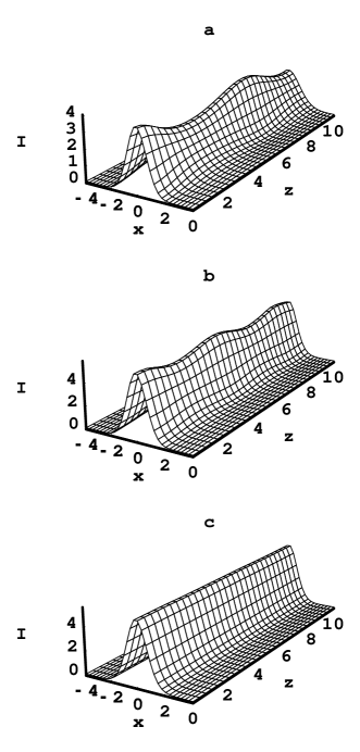
Figure 2: The propagations of light beams in nonlocal media with a Gaussian function type nonlocal response with different input intensity profiles that are described by (a) $|u_{0}(x,0)|^{2}$ in Eq. (22), (b) $|\psi_{0}(A,0,0,x)|^{2}$ and (c) $|\psi_{0}(A,\alpha,\beta,x)|^{2}$ respectively. Here $w_{0}=2,\mu=1,\nu=1,A=3.217,\alpha=-0.0487,\beta=0.00317$ and the degree of nonlocality $w_{0}/\mu=2$.

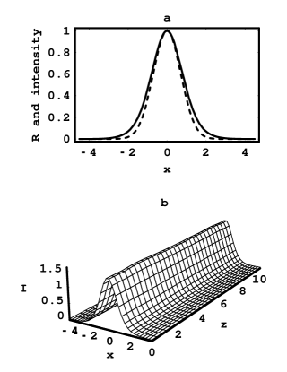
Figure 3: (a) The comparison between $R(x)$ and $|\psi_{0}(A,\alpha,\beta,x)|^{2}$. Dashing line: $R(x)/R(0)$; solid line: $|\psi_{0}(A,\alpha,\beta,x)|^{2}/|\psi_{0}(A,\alpha,\beta,0)|^{2}$; (b)The propagation of the light beam with an input intensity profile described by $|\psi_{0}(A,\alpha,\beta,x)|^{2}$. Here $w_{0}=1,\mu=1,A=1.777,\alpha=-0.113,\beta=0.0177$ and the degree of nonlocality $w_{0}/\mu=1$.

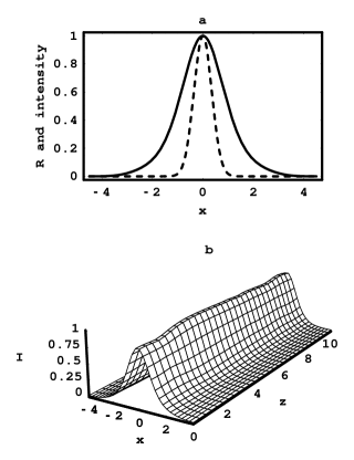
Figure 4: (a) The comparison between $R(x)$ and $|\psi_{0}(A,\alpha,\beta,x)|^{2}$. Dashing line: $R(x)/R(0)$; solid line: $|\psi_{0}(A,\alpha,\beta,x)|^{2}/|\psi_{0}(A,\alpha,\beta,0)|^{2}$; (b)The propagation of the light beam with an input intensity profile described by $|\psi_{0}(A,\alpha,\beta,x)|^{2}$. Here $w_{0}=0.5,\mu=1,A=1.403,\alpha=-0.178,\beta=0.0476$ and the degree of nonlocality $w_{0}/\mu=0.5$

Table 1: Using the numerical simulation method we calculate $\bar{\theta}$ in Eqs. (26) for the nonlocal case of the Gaussian function type nonlocal response and for the nonlocal case of the exponential-decay type nonlocal response.

		$\bar{\theta}$
$\psi_{0}$	0.020	0.0033	0.0027	0.0027	0.0026	0.0026	0.0026
$\psi_{1}$	0.044	0.013	0.013	0.013	0.013	0.013	0.013
$\psi_{0}$	0.017	0.0095	0.0078	0.0072	0.0071	0.0069	0.0068
$\psi_{1}$	0.072	0.044	0.037	0.034	0.032	0.031	0.031
$\psi_{2}$	0.36	0.20	0.17	0.15	0.14	0.14	0.13

Now let us consider the properties of $\psi_{0}(A,\alpha,\beta,x)$. As have been shown, the beam width of $\psi_{0}(A,\alpha,\beta,x)$ is approximatively given by $\mu$, and its power and phase constant are approximatively given by

$$P\approx A^{2}\approx{{\sqrt{\pi}(1+w_{0}^{2}/\mu^{2})^{3/2}}\over{2\mu}},$$ (27)

$$\gamma=-V_{0}-\varepsilon_{0}~{}~{}~{}~{}~{}~{}~{}~{}~{}~{}~{}~{}~{}~{}~{}~{}~{}~{}~{}~{}~{}~{}~{}~{}~{}~{}~{}~{}~{}~{}~{}~{}~{}~{}~{}~{}~{}~{}~{}~{}$$

$$\approx{{1}\over{2\mu^{2}}}\left[{{w_{0}^{2}}\over{\mu^{2}}}+{{3}\over{8(1+w_{0}^{2}/\mu^{2})}}+{{1}\over{64(1+w_{0}^{2}/\mu^{2})^{2}}}\right]$$ (28)

respectively. In the strongly nonlocal limit the degree of nonlocality $w_{0}/\mu\gg 1$, we have

$$P\approx{{\sqrt{\pi}w_{0}^{3}}\over{2\mu^{4}}},$$ (29)

$$\gamma\approx{{w_{0}^{2}}\over{2\mu^{4}}}.$$ (30)

That means for a given value of characteristic nonlocal length in the strongly nonlocal case the power and the phase constant of the nonlocal soliton are both in inverse proportion to the 4th power of its beam width. The dependence of the power $P$ and the phase constant $\gamma$ on the beam width $\mu$ are shown in Fig. (5) for a given value of characteristic nonlocal length. It is indicated that Eq. (27) and Eq. (30) can describe these dependence exactly in the generally nonlocal case.

To make a comparison with the local soliton, let us consider the following local nonlinear Schrödinger equation(NLSE)a

$$i{{\partial u}\over{\partial z}}+{{1}\over{2}}{{\partial^{2}u}\over{\partial x^{2}}}+|u|^{2}u=0.$$ (31)

When the characteristic nonlocal length $w_{0}$ approaches zero, the Gaussian function type nonlocal response function $R(x)$ approaches the $\delta(x)$ function, and the NNLSE (1) approaches the NLSE (31). The fundamental soliton of the NLSE (31) is given bya

$$u(x,z)={{1}\over{\eta}}sech({{x}\over{\eta}})\exp\left(i{{z}\over{2\eta^{2}}}\right),$$ (32)

where $\eta$ can be viewed as the beam width of the local soliton. The power and the phase constant of such a local soliton are given by

$$P=\int^{+\infty}_{-\infty}|u(x,t)|^{2}dx={{2}\over{\eta}},$$ (33)

$$\gamma={{1}\over{2\eta^{2}}}$$ (34)

respectively. We can find the power and the phase constant of the local soliton are in inverse proportion to the 1st and the 2nd power of its beam width respectively. The functional dependence of the power and the phase constant of the nonlocal soliton on its beam width greatly differs from that of the local soltion.

Figure 5: The dependence of the power $P$ and the phase constant $\gamma$ on the beam width $\mu$. Dashing lines are described by Eq. (27) and Eq. (30) respectively; Thin solid line is described by Eq. (29); Thick solid lines are directly calculated with parameters $A,\alpha,\beta$ numerically found by the fixed-point method presented in the section Appendix (A). Here $w_{0}=6$.

II.2 the nonlocal case of an exponential-decay type nonlocal response

As another example, we investigate the nonlocal case where the light-induced perturbed refractive index $n(x,z)$ is governed by11 ; 10 ; 17

$$n(x,z)-w_{0}^{2}{{\partial^{2}n(x,z)}\over{\partial x^{2}}}-|u(x,z)|^{2}=0.$$ (35)

It is found that several nonlocal media, for example the nematic liquid crystal5 ; 17 , their light-induced perturbed refractive index can be described by Eq. (35). If the size of the nonlocal media is much larger than the beam width of the soliton and the characteristic nonlocal length, the effect of the boundary condition on the soliton can be negligible and we can simply assume the size of the nonlocal media is infinity large. For such a case, equation (35) leads

$$n(x,z)={{1}\over{2w_{0}}}\int^{+\infty}_{-\infty}\exp\left(-{{|x-\xi|}\over{w_{0}}}\right)|u(\xi,z)|^{2}d\xi,$$ (36)

and we get the exponential-decay type nonlocal response1 ; 13 ; 10 ; 11 ; 14

$$R(x)={{1}\over{2w_{0}}}\exp\left(-{{|x|}\over{w_{0}}}\right).$$ (37)

Since the exponential-decay type nonlocal response function $R(x)$ is not differentiable at $x=0$, the SNM (3) can’t deal with this nonlocal case. So we have to use $\psi_{0}(A,\alpha,\beta,x)$ to describe the soliton state of the NNLSE (1).

For this exponential-decay type nonlocal response and the fundamental soliton state, $V(x)$ can be approximately given by

$$V(x)\approx-\int^{+\infty}_{-\infty}{{1}\over{2w_{0}}}\exp\left(-{{|x-\xi|}\over{w_{0}}}\right)|\psi_{0}(A,0,0,\xi)|^{2}d\xi~{}$$

$$={{A^{2}}\over{4w_{0}}}e^{{\mu^{2}}\over{4w_{0}^{2}}}\{e^{-{{x}\over{w_{0}}}}[erf\left({{\mu}\over{2w_{0}}}-{{x}\over{\mu}}\right)-1]~{}~{}$$

$$+e^{{x}\over{w_{0}}}[erf\left({{\mu}\over{2w_{0}}}+{{x}\over{\mu}}\right)-1]\},$$ (38)

where

$$erf(x)={{2}\over{\sqrt{\pi}}}\int^{x}_{0}e^{-\xi^{2}}d\xi.$$ (39)

Combining Eqs. (12), we get

$$A^{2}\approx{{1/\mu}\over{{{\mu^{2}}\over{\sqrt{\pi}w_{0}^{2}}}+\exp({{\mu^{2}}\over{4w_{0}^{2}}}){{\mu^{3}}\over{2w_{0}^{3}}}[erf({{\mu}\over{2w_{0}}})-1]}},$$ (40a)

$$V_{0}\approx-{{A^{2}\exp({{\mu^{2}}\over{4w_{0}^{2}}})[1-erf({{\mu}\over{2w_{0}}})]}\over{2w_{0}}},$$ (40b)

$$\alpha\approx{{A^{2}\{\exp({{\mu^{2}}\over{4w_{0}^{2}}})[erf({{\mu}\over{2w_{0}}})-1]+{{2w_{0}}\over{\sqrt{\pi}\mu}}-{{4w_{0}^{3}}\over{\sqrt{\pi}\mu^{3}}}\}}\over{48w_{0}^{5}}},$$ (40c)

$$\beta\approx{{A^{2}\{\exp({{\mu^{2}}\over{4w_{0}^{2}}})[erf({{\mu}\over{2w_{0}}})-1]+{{2w_{0}}\over{\sqrt{\pi}\mu}}-{{4w_{0}^{3}}\over{\sqrt{\pi}\mu^{3}}}+{{24w_{0}^{5}}\over{\sqrt{\pi}\mu^{5}}}\}}\over{1440w_{0}^{7}}}.$$ (40d)

In the strongly nonlocal limit the degree of nonlocality $w_{0}/\mu\gg 1$, we obtain

$$A^{2}\approx{{\sqrt{\pi}w_{0}^{2}}\over{\mu^{3}}},$$ (41a)

$$V_{0}\approx-{{\sqrt{\pi}w_{0}}\over{2\mu^{3}}},$$ (41b)

$$\alpha\approx-{{1}\over{12\mu^{6}}},$$ (41c)

$$\beta\approx{{1}\over{60\mu^{8}}}.$$ (41d)

It is worth to note that in the strongly nonlocal case the parameters $\alpha$ and $\beta$ are free from the characteristic nonlocal length $w_{0}$. Even when the characteristic nonlocal length $w_{0}$ approaches infinity, the parameters $\alpha,\beta$ still rest on finite values and don’t approach zero, and therefore $\psi_{0}(A,\alpha,\beta,x)$ does’t approach $\psi_{0}(A,0,0,x)$. That greatly differs from the nonlocal case of a Gaussian function type nonlocal response. As a result the Gaussian-function-like soliton solution $\psi_{0}(A,0,0,x)$ can’t describe the soliton state of the NNLSE (1) exactly even in the strongly nonlocal case, that is shown in Fig. (6). As shown in Fig. (7), $\psi_{0}(A,\alpha,\beta,x)$ also can describe the soliton state of the NNLSE (1) exactly when $w_{0}/\mu=1$. Even when $w_{0}/\mu=0.5$, as indicated in Fig. (8), $\psi_{0}(A,\alpha,\beta,x)$ can describe the soliton state of the NNLSE (1) in high quality. As indicated by the values of $\bar{\theta}$ in table (1), $\psi_{0}(A,\alpha,\beta,x)$ can describe the fundamental soliton states of NNLSE (1) exactly in the generally nonlocal case.

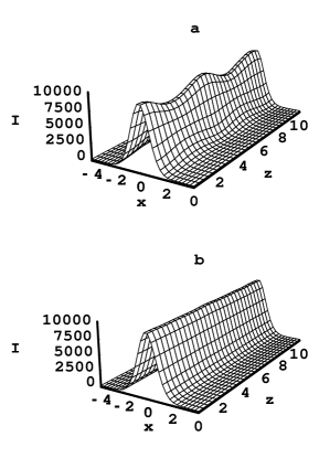
Figure 6: The propagations of light beams with different input intensity profiles that are described by (a) $|\psi_{0}(A,0,0,x)|^{2}$ and (b) $|\psi_{0}(A,\alpha,\beta,x)|^{2}$ respectively. Here $w_{0}=100,\mu=1,A=138.159,\alpha=-0.0767,\beta=0.0150$ and the degree of nonlocality $w_{0}/\mu=100$.

Figure 7: (a) The comparison between $R(x)$ and $|\psi_{0}(A,\alpha,\beta,x)|^{2}$. Dashing line: $R(x)/R(0)$; solid line: $|\psi_{0}(A,\alpha,\beta,x)|^{2}/|\psi_{0}(A,\alpha,\beta,0)|^{2}$; (b)The propagation of the light beam with an input intensity profile described by $|\psi_{0}(A,\alpha,\beta,x)|^{2}$. Here $w_{0}=1,\mu=1,A=2.206,\alpha=-0.126,\beta=0.0280$ and the degree of nonlocality $w_{0}/\mu=1$.

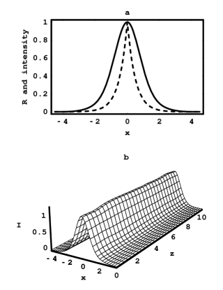
Figure 8: (a) The comparison between $R(x)$ and $|\psi_{0}(A,\alpha,\beta,x)|^{2}$. Dashing line: $R(x)/R(0)$; solid line: $|\psi_{0}(A,\alpha,\beta,x)|^{2}/|\psi_{0}(A,\alpha,\beta,0)|^{2}$; (b) The propagation of the light beam with an input intensity profile described by $|\psi_{0}(A,\alpha,\beta,x)|^{2}$. Here $w_{0}=0.5,\mu=1,A=1.610,\alpha=-0.158,\beta=0.0408$ and the degree of nonlocality $w_{0}/\mu=0.5$.

In the strongly nonlocal case the soliton’s power and phase constant are approximately given by

$$P\approx A^{2}\approx{{\sqrt{\pi}w_{0}^{2}}\over{\mu^{3}}},$$ (42)

$$\gamma\approx-V_{0}\approx{{\sqrt{\pi}w_{0}}\over{2\mu^{3}}}$$ (43)

respectively. For a given value of the characteristic nonlocal length, the soliton’s power and phase constant are both in inverse proportion to the 3th power of its beam width in the strongly nonlocal case that differs from the nonlocal case of a Gaussian function type nonlocal response where the soliton’s power and phase constant are both in inverse proportion to the 4th power of its beam width in the strongly nonlocal case. The dependence of the soliton’s power $P$ and phase constant $\gamma$ on its beam width $\mu$ are shown in Fig. (9) for a given value of characteristic nonlocal length. It is indicated that Eq. (42) and Eq. (43) can describe these dependence very well in the strongly nonlocal case.

Figure 9: The dependence of the soliton’s power $P$ and phase constant $\gamma$ on its beam width $\mu$. Dashing lines are described by Eq. (42) and Eq. (43) respectively; Solid lines are directly calculated with parameters $A,\alpha,\beta$ numerically found by the fixed-point method presented in the section Appendix (A). Here $w_{0}=6$.

III the higher order generally nonlocal soliton solutions in the 2nd approximation

III.1 the nonlocal case of the Gaussian function type nonlocal response

The second order soliton solution for the SNM (3) is given by

$$u_{1}(x,z)=A\left({{1}\over{\pi\nu^{2}}}\right)^{1/4}{{\sqrt{2}x}\over{\nu}}e^{-{{x^{2}}\over{2\nu^{2}}}-i({{9}\over{4\nu^{2}}}-R_{0}A^{2})z},$$ (44)

where

$${{1}\over{\nu^{4}}}=-R^{\prime\prime}_{0}A^{2}.$$ (45)

The power and the beam width of $u_{1}(x,z)$ are given by $A^{2}$ and $\sqrt{3}\nu$ respectively. For the Gaussian function type nonlocal response, the second order soliton solution for the SNM (3) is given by

$$u_{1}(x,z)=({{\sqrt{\pi}w_{0}^{3}}\over{2\nu^{4}}})^{{{1}\over{2}}}({{1}\over{\pi\nu^{2}}})^{{{1}\over{4}}}{{\sqrt{2}x}\over{\nu}}e^{-{{x^{2}}\over{2\nu^{2}}}-i({{9}\over{4\nu^{2}}}-{{w_{0}^{2}}\over{2\nu^{4}}})z}.$$ (46)

This soliton solution can describe the second order soliton state of the NNLSE (1) exactly in the strongly nonlocal case when $w_{0}/(\sqrt{3}\nu)>10$ but can’t describe it exactly in the generally nonlocal case when $w_{0}/(\sqrt{3}\nu)\sim 2$.

The second order generally nonlocal soliton solution in the 2nd approximation is given by

$$\psi_{1}(A,\alpha,\beta,x)\approx A({{1}\over{\pi\mu^{2}}})^{1/4}\exp(-{{x^{2}}\over{2\mu^{2}}}){{\sqrt{2}x}\over{\mu}}~{}~{}~{}~{}~{}~{}$$

$$\times[1+\alpha({{45\mu^{6}}\over{16}}-{{5\mu^{4}}\over{4}}x^{2}-{{\mu^{2}}\over{4}}x^{4})~{}~{}~{}~{}~{}~{}~{}~{}~{}~{}~{}~{}~{}~{}~{}~{}~{}~{}~{}$$

$$+\alpha^{2}(-{{8375\mu^{12}}\over{512}}+{{215\mu^{10}}\over{64}}x^{2}+{{73\mu^{8}}\over{64}}x^{4}+{{19\mu^{6}}\over{48}}x^{6}+{{\mu^{4}}\over{32}}x^{8})$$

$$+\beta({{385\mu^{8}}\over{32}}-{{35\mu^{6}}\over{8}}x^{2}-{{7\mu^{4}}\over{8}}x^{4}-{{\mu^{2}}\over{6}}x^{6})],~{}~{}~{}~{}~{}~{}~{}~{}~{}~{}~{}$$ (47)

and

$$\varepsilon_{1}\approx{{3}\over{2\mu^{2}}}+{{15\alpha\mu^{4}}\over{4}}-{{165\alpha^{2}\mu^{10}}\over{8}}+{{105\beta\mu^{6}}\over{8}}.$$ (48)

For the Gaussian function type nonlocal response function (21), as shown in Fig. (10), the difference between $|\psi_{1}(A,\alpha,\beta,x)|^{2}$ and $|\psi_{1}(A,0,0,x)|^{2}$ is small in the generally nonlocal case. As an Hermite-Gaussian function, the power and the beam width of $\psi_{1}(A,0,0,x)$ are given by $A^{2}$ and $\sqrt{3}\mu$ respectively. So the power and the beam width of $\psi_{1}(A,\alpha,\beta,x)$ are also approximatively given by $A^{2}$ and $\sqrt{3}\mu$ respectively. We can approximatively determine the degree of nonlocality by $w_{0}/(\sqrt{3}\mu)$ and approximatively abtain

$$V(x)\approx-\int^{+\infty}_{-\infty}{{1}\over{w_{0}\sqrt{\pi}}}\exp\left[-{{(x-\xi)^{2}}\over{w_{0}^{2}}}\right]\psi_{1}^{2}(A,0,0,\xi)d\xi$$

$$=-{{A^{2}}\over{\sqrt{\pi(\mu^{2}+w_{0}^{2})}}}e^{-{{x^{2}}\over{\mu^{2}+w_{0}^{2}}}}{{2x^{2}/\mu^{2}+w_{0}^{2}/\mu^{2}+w_{0}^{4}/\mu^{4}}\over{(1+w_{0}^{2}/\mu^{2})^{2}}},$$ (49)

and

$$A^{2}\approx{{\sqrt{\pi}(1+w_{0}^{2}/\mu^{2})^{5/2}}\over{2\mu(w_{0}^{2}/\mu^{2}-2)}},$$ (50a)

$$V_{0}\approx-{{w_{0}^{2}(1+w_{0}^{2}/\mu^{2})}\over{2\mu^{4}(w_{0}^{2}/\mu^{2}-2)}},$$ (50b)

$$\alpha\approx-{{(w_{0}^{2}/\mu^{2}-4)}\over{4\mu^{6}(1+w_{0}^{2}/\mu^{2})(w_{0}^{2}/\mu^{2}-2)}},$$ (50c)

$$\beta\approx{{(w_{0}^{2}/\mu^{2}-6)}\over{12\mu^{8}(1+w_{0}^{2}/\mu^{2})^{2}(w_{0}^{2}/\mu^{2}-2)}}.$$ (50d)

In the strongly nonlocal limit the degree of nonlocality $w_{0}/(\sqrt{3}\mu)\gg 1$, we have

$$A^{2}\approx{{\sqrt{\pi}w_{0}^{3}}\over{2\mu^{4}}},$$ (51a)

$$V_{0}\approx-{{w_{0}^{2}}\over{2\mu^{4}}},$$ (51b)

$$\alpha\approx-{{1}\over{4\mu^{4}w_{0}^{2}}},$$ (51c)

$$\beta\approx{{1}\over{12\mu^{4}w_{0}^{4}}}.$$ (51d)

As the degree of nonlocality $w_{0}/(\sqrt{3}\mu)$ approaches infinity, the parameters $\alpha$ and $\beta$ approach zero, and $\psi_{1}(A,\alpha,\beta,x)$ approaches $\psi_{1}(A,0,0,x)$. Therefore in the strongly nonlocal case an Hermite-Gaussian-function-like second order soliton solution is obtained, and the power and the phase constant of $\psi_{1}(A,\alpha,\beta,x)$ are both in inverse proportion to the 4th power of its beam width. As indicated in Fig. (11) and Fig. (12), the second order soliton solution in the 2nd perturbation $\psi_{1}(A,\alpha,\beta,x)$ can describe the second order soliton state of the NNLSE (1) exactly when $w_{0}/(\sqrt{3}\mu)=1.5$ and describe it in high qulity when $w_{0}/(\sqrt{3}\mu)=1$. As shown by the values of $\bar{\theta}$ in table (1),$\psi_{1}(A,\alpha,\beta,x)$ can exactly describe the second order nonlocal soltion state in the generally nonlocal cases.

Finally since the all eigenfunctions of the harmonic oscillator can be found systematically24 , it is possible that in analogy to a perturbed harmonic oscillator we can also approximately calculate the third order soliton solution or the fourth order soliton solution and so on in the generally nonlocal case for the Gaussian function type nonlocal response.

Figure 10: The comparison between $|\psi_{1}(A,\alpha,\beta,x)|^{2}$ (dashing line) and $|\psi_{1}(A,0,0,x)|^{2}$ (solid line). Here $w_{0}=1.5,\mu=1/\sqrt{3},A=7.606,\alpha=-0.450,\beta=0.00530$ and the degree of nonlocality $w_{0}/(\sqrt{3}\mu)=1.5$.

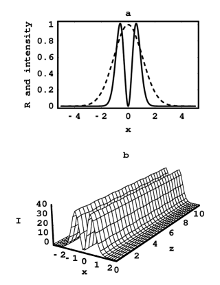
Figure 11: (a) The comparison between $R(x)$ and $|\psi_{1}(A,\alpha,\beta,x)|^{2}$. Dashing line: $R(x)/R(0)$; solid line: $|\psi_{1}(A,\alpha,\beta,x)|^{2}/|\psi_{1}(A,\alpha,\beta,0.65)|^{2}$; (b)The propagation of the light beam with an input intensity profile described by $|\psi_{1}(A,\alpha,\beta,x)|^{2}$. Here $w_{0}=1.5,\mu=1/\sqrt{3},A=7.606,\alpha=-0.450,\beta=0.00530$ and the degree of nonlocality $w_{0}/(\sqrt{3}\mu)=1.5$.

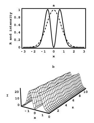
Figure 12: (a) The comparison between $R(x)$ and $|\psi_{1}(A,\alpha,\beta,x)|^{2}$. Dashing line: $R(x)/R(0)$; solid line: $|\psi_{1}(A,\alpha,\beta,x)|^{2}/|\psi_{1}(A,\alpha,\beta,0.65)|^{2}$; (b)The propagation of the light beam with an input intensity profile described by $|\psi_{1}(A,\alpha,\beta,x)|^{2}$. Here $w_{0}=1,\mu=1/\sqrt{3},A=6.133,\alpha=-0.492,\beta=0.0145$ and the degree of nonlocality $w_{0}/(\sqrt{3}\mu)=1$.

III.2 the nonlocal case of the exponential-decay type nonlocal response

As have been indicated, to $\psi_{0}(A,\alpha,\beta,x)$ and $\psi_{1}(A,\alpha,\beta,x)$ in the nonlocal case of the Gaussian function type nonlocal response and to $\psi_{0}(A,\alpha,\beta,x)$ in the nonlocal case of the exponential-decay type nonlocal response, we have $V^{(2)}(A,\alpha,\beta,0)>0$ for generally nonlocal cases. If we define

$$\tilde{V}(x)=V_{0}+{{1}\over{2\mu^{4}}}x^{2}+\alpha x^{4}+\beta x^{6},$$ (52)

we will get $V(A,\alpha,\beta,x)\approx\tilde{V}(x)$. But as shown in Figs. (13a) and (14a), to $\psi_{1}(A,\alpha,\beta,x)$ in the nonlocal case of the exponential-decay type nonlocal response, we have $V^{(2)}(A,\alpha,\beta,0)<0$. In such a case we can’t define $1/\mu^{4}=V^{(2)}(A,\alpha,\beta,0)$ and can’t define the parameters $\mu,\alpha,\beta$ as those in Eqs. (20). However as shown in Figs. (13a) and (14a), we still can find suitable values of $A,\alpha,\beta$ for a fixed value of $\mu$ to make $V(A,\alpha,\beta,x)\approx\tilde{V}(x)$. These suitable values of $A,\alpha,\beta$ can be calculated by solving the following coupling equations

$$V(A,\alpha,\beta,x_{0})=V_{0}+{{1}\over{2\mu^{4}}}x_{0}^{2}+\alpha x_{0}^{4}+\beta x_{0}^{6},$$ (53a)

$$V^{\prime}(A,\alpha,\beta,x_{0})={{1}\over{\mu^{4}}}x_{0}+4\alpha x_{0}^{3}+6\beta x_{0}^{5},$$ (53b)

$$V^{\prime\prime}(A,\alpha,\beta,x_{0})={{1}\over{\mu^{4}}}+12\alpha x_{0}^{2}+30\beta x_{0}^{4},$$ (53c)

where $x_{0}\neq 0$ and $V_{0}=V(A,\alpha,\beta,0)$. In the section Appendix (B) we present a fixed-point method to calculate these parameters $A,\alpha,\beta$ with Eqs. (53). In Figs. (13b),(14b) and (15b) we show the propagation of lights with input intensity profiles described by $|\psi_{1}(A,\alpha,\beta,x)|^{2}$. Even when the $w_{0}/(\sqrt{3}\mu)=0.5$, there still exists a second order nonlocal soliton. As shown by the values of $\bar{\theta}$ in table (1), $\psi_{1}(A,\alpha,\beta,x)$ can describe the generally nonlocal soliton state in high quality. Since the difference between $\psi_{1}(A,\alpha,\beta,x)$ and $\psi_{1}(A,0,0,x)$ is small, we can approximately get

$$V(x)\approx-\int^{+\infty}_{-\infty}{{1}\over{2w_{0}}}\exp\left(-{{|x-\xi|}\over{w_{0}}}\right)|\psi_{1}(A,0,0,\xi)|^{2}d\xi~{}$$

$$={{A^{2}}\over{8w_{0}}}({{\mu^{2}}\over{w_{0}^{2}}}+2)e^{{\mu^{2}}\over{4w_{0}^{2}}}\{e^{-{{x}\over{w_{0}}}}[erf({{\mu}\over{2w_{0}}}-{{x}\over{\mu}})-1]~{}~{}$$

$$+e^{{x}\over{w_{0}}}[erf({{\mu}\over{2w_{0}}}+{{x}\over{\mu}})-1]\}+{{A^{2}\mu}\over{2\sqrt{\pi}w_{0}^{2}}}e^{-{{x^{2}}\over{\mu^{2}}}}.$$ (54)

By defining

$$U(x)=V(x)/A^{2}$$ (55)

and combining with Eqs. (53), we obtain

$$A\approx\sqrt{{{4x_{0}^{2}/\mu^{4}}\over{24[U(x_{0})-U(0)]-9U^{\prime}(x_{0})x_{0}+U^{\prime\prime}(x_{0})x_{0}^{2}}}}.$$ (56)

For example, when $w_{0}=10,\mu=1/\sqrt{3},x_{0}=2$, from Eqs. (54), (55) and (56) we get $A\approx 47.323$ that is close to the numerically calculated value $A=48.257$.

While $V(A,\alpha,\beta,x)\approx\tilde{V}(x)$, as shown in Figs. (13a) and (14a) there still exists difference $H(x)=V(A,\alpha,\beta,x)-\tilde{V}(x)$. To achieve higher accuracy we should take $H(x)$ into account and set $\tilde{V}(x)=V_{0}+x^{2}/(2\mu^{2})+\alpha x^{4}+\beta x^{6}+H(x)$. Viewing $H(x)$ as perturbation we will obtain another higher accurate second order soliton solution. However the form of $H(x)$ is rather complex and we will leave it in future further work and don’t intent to deal with the effect of $H(x)$ in this paper.

Figure 13: (a) The comparison between $V(A,\alpha,\beta,x)$ (solid line) and $\tilde{V}(x)$ (dashing line); (b)The propagation of the light beam with an input intensity profile described by $|\psi_{1}(A,\alpha,\beta,x)|^{2}$. Here $w_{0}=2,\mu=1/\sqrt{3},A=12.162,\alpha=-0.442,\beta=0.0179$ and the degree of nonlocality $w_{0}/(\sqrt{3}\mu)=2$.

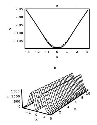
Figure 14: (a) The comparison between $V(A,\alpha,\beta,x)$ (solid line) and $\tilde{V}(x)$ (dashing line); (b)The propagation of the light beam with an input intensity profile described by $|\psi_{1}(A,\alpha,\beta,x)|^{2}$. Here $w_{0}=10,\mu=1/\sqrt{3},A=48.257,\alpha=-0.348,\beta=0.0141$ and the degree of nonlocality $w_{0}/(\sqrt{3}\mu)=10$.

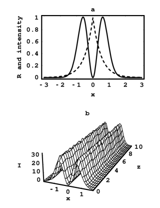
Figure 15: (a) The comparison between $R(x)$ and $|\psi_{1}(A,\alpha,\beta,x)|^{2}$. Dashing line: $R(x)/R(0)$; solid line: $|\psi_{1}(A,\alpha,\beta,x)|^{2}/|\psi_{1}(A,\alpha,\beta,0.65)|^{2}$; (b)The propagation of the light beam with an input intensity profile described by $|\psi_{1}(A,\alpha,\beta,x)|^{2}$. Here $w_{0}=0.5,\mu=1/\sqrt{3},A=6.303,\alpha=-0.609,\beta=0.0270$ and the degree of nonlocality $w_{0}/(\sqrt{3}\mu)=0.5$.

Now let us consider the third order nonlocal soliton. The third order generally nonlocal soliton solution in the 2nd approximation is given by

$$\psi_{2}(A,\alpha,\beta,x)\approx A({{1}\over{\pi\mu^{2}}})^{1/4}\exp(-{{x^{2}}\over{2\mu^{2}}}){{1}\over{\sqrt{2}}}[-1+{{2x^{2}}\over{\mu^{2}}}$$

$$+\alpha(-{{45\mu^{6}}\over{16}}+{{123\mu^{4}}\over{8}}x^{2}-{{13\mu^{2}}\over{4}}x^{4}-{{1}\over{2}}x^{6})+\alpha^{2}({{11927\mu^{12}}\over{512}}$$

$$-{{24587\mu^{10}}\over{256}}x^{2}+{{41\mu^{8}}\over{64}}x^{4}+{{193\mu^{6}}\over{96}}x^{6}+{{97\mu^{4}}\over{96}}x^{8}+{{\mu^{2}}\over{16}}x^{10})$$

$$+\beta(-{{655\mu^{8}}\over{32}}+{{1405\mu^{6}}\over{16}}x^{2}-{{125\mu^{4}}\over{8}}x^{4}-{{25\mu^{2}}\over{12}}x^{6}-{{1}\over{3}}x^{8})].$$ (57)

As shown in Fig. (16) and table (1),$\psi_{1}(A,\alpha,\beta,x)$ can describe the third order generally nonlocal soliton only qualitatively. To obtain a higher accurate third order soliton solution we should take all perturbation into account or develop another new method.

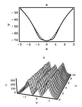
Figure 16: (a) The comparison between $V(A,\alpha,\beta,x)$ (solid line) and $\tilde{V}(x)$ (dashing line); (b)The propagation of the light beam with an input intensity profile described by $|\psi_{2}(A,\alpha,\beta,x)|^{2}$. Here $w_{0}=2,\mu=1/\sqrt{5},A=19.694,\alpha=-1.327,\beta=0.0606$ and the degree of nonlocality $w_{0}/(\sqrt{5}\mu)=2$.

IV Conclusion

In analogy to a perturbed harmonic oscillator, we calculate the fundamental and some other higher order soliton solutions in the 2nd approximation in the generally nonlocal case. Numerical simulations confirm that the soliton solutions in the 2nd perturbation can describe the fundamental and second order soliton states of the NNLSE (1) in high quality. For the nonlocal case of the exponential-decay type nonlocal response, the Gaussian-function-like soliton solution can’t describe the fundamental soliton state of the NNLSE (1) exactly even in the strongly nonlocal case, that greatly differs from the nonlocal case of the Gaussian function type nonlocal response. The functional dependence of the nonlocal soliton’s power and phase constant on its beam width are greatly different from that of the local soliton. In the strongly nonlocal case, the soltion’s power and phase constant are both in inverse proportion to the 4th power of its beam width for the nonlocal case of the Gaussian function type nonlocal response, and are both in inverse proportion to the 3th power of its beam width for the nonlocal case of the exponential-decay type nonlocal response.

Appendix A how to calculate the parameters $A,\alpha,\beta$ with equations. (20)

In principle, $V(A,\alpha,\beta,x)$ and the parameters $A,\alpha,\beta$ can be found by solving Eq. (19) and Eqs. (20) directly, but these tasks are considerably involved. Here we present a fixed-point method to calculate these parameters $A,\alpha,\beta$ for a fixed value of $\mu$. Firstly corresponding to $V(A,\alpha,\beta,x)$ in Eq. (19), we define

$$U(\alpha,\beta,x)={{V(A,\alpha,\beta,x)}\over{A^{2}}}.$$ (58)

For an arbitrary pair of initial values of $\alpha_{0},\beta_{0}$ with suitable order of the magnitude, we can calculate $U(\alpha_{0},\beta_{0},x)$. Let

$$A_{1}=\sqrt{{{1}\over{\mu^{4}U^{(2)}(\alpha_{0},\beta_{0},0)}}},$$ (59)

$$\alpha_{1}=A_{1}^{2}U^{(4)}(\alpha_{0},\beta_{0},0)/4!,$$ (60)

$$\beta_{1}=A_{1}^{2}U^{(6)}(\alpha_{0},\beta_{0},0)/6!.$$ (61)

For such a pair of values of $\alpha_{1},\beta_{1}$, we can find another $U(\alpha_{1},\beta_{1},x)$. Again we obtain another set of values $\{A_{2},\alpha_{2},\beta_{2}\}$. Repeating these steps of calculations, we can obtain series sets of values $\{A_{2},\alpha_{3},\beta_{3}\}$, $\{A_{3},\alpha_{4},\beta_{4}\}$, and so on. The difference between $\{A_{m},\alpha_{m},\beta_{m}\}$ and $\{A_{m+1},\alpha_{m+1},\beta_{m+1}\}$ will approaches zero as the number of $m$ approaches infinity. To some accuracy, we can calculate parameters $A,\alpha,\beta$ for a fixed value of $\mu$.

Appendix B how to calculate the parameters $A,\alpha,\beta$ with equations. (53)

For a fixed value of $\mu$ and one suitable point $x_{0}\neq 0$ (in this paper we set $x_{0}=2$), corresponding to $V(A,\alpha,\beta,x)$ in Eq. (19) we define

$$U(x)={{V(A,\alpha,\beta,x)}\over{A^{2}}}.$$ (62)

For an arbitrary pair of initial values of $\alpha_{0},\beta_{0}$ with suitable order of the magnitude, we can calculate $U(x)$. Let

$$A_{1}=\sqrt{{{4x_{0}^{2}/\mu^{4}}\over{24[U(x_{0})-U(0)]-9U^{\prime}(x_{0})x_{0}+U^{\prime\prime}(x_{0})x_{0}^{2}}}},$$ (63)

$$\alpha_{1}=A_{1}^{2}{{7U^{\prime}(x_{0})x_{0}-12[U(x_{0})-U(0)]-U^{\prime\prime}(x_{0})x_{0}^{2}}\over{4x_{0}^{4}}},$$ (64)

$$\beta_{1}=A_{1}^{2}{{U^{\prime\prime}(x_{0})x_{0}^{2}+8[U(x_{0})-U(0)]-5U^{\prime}(x_{0})x_{0}}\over{8x_{0}^{6}}}.$$ (65)

For such a pair of values of $\alpha_{1},\beta_{1}$, we can find another $U(x)$. Again we obtain another set of values $\{A_{2},\alpha_{2},\beta_{2}\}$. Repeating these steps of calculations, to some accuracy we can calculate parameters $A,\alpha,\beta$ for a fixed value of $\mu$.

References

• (1) A. W. Snyder and D. J. Mitchell, Science, $\bf{276}$, 1538 (1997).
• (2) W. Krolikowski and O. Bang, Phys. Rev. E $\bf{63}$, 016610 (2000).
• (3) Q. Guo, B. Luo, F. Yi, S. Chi and Y. Xie, Phys. Rev. E $\bf{69}$, 016602 (2004).
• (4) N.I. Nikolov, D. Neshev, W. Krolikowski, O. Bang, J.J. Rasmussen and P.L. Christiansen, Opt. Lett. $\bf{29}$, 286 (2004).
• (5) Y. Huang, Q. Guo and J. Cao, Opt. Comm. $\bf{261}$, 175 (2006).
• (6) D.J. Mitchell and A.W. Snyder, J.Opt.Soc.Am.B $\bf{16}$, 236 (1999).
• (7) W.Krolikowski, O. Bang and J.Wyller, Phys. Rev. E $\bf{70}$, 036617 (2004).
• (8) S. Abe and A. Ogura, Phys. Rev. E $\bf{57}$, 6066 (1998).
• (9) W. Krolikowski, O. Bang, J.J. Rasmussen and J. Wyller, Phys. Rev. E $\bf{64}$, 016612 (2001).
• (10) J. Wyller, W. Krolikowski, O. Bang and J.J. Rasmussen, Phys. Rev. E $\bf{66}$, 066615 (2002).
• (11) O. Bang, W. Krolikowski, J. Wyller and J. J. Rasmussen, Phys. Rev. E $\bf{66}$, 046619 (2002).
• (12) N.I. Nikolov, D. Neshev, O. bang and W. Krolikowski, Phys. Rev. E $\bf{68}$, 036614 (2003).
• (13) Y. Xie and Q. Guo, Optical and Quantum Electronics, $\bf{36}$, 1335 (2004).
• (14) Q. Guo, B. Luo and S. Chi, Opt. Comm. $\bf{259}$, 336 (2006).
• (15) C. Conti, M. Peccianti and G. Assanto, Phys. Rev. Lett. $\bf{91}$, 073901 (2003).
• (16) M. Peccianti, C. Conti and G. Assanto, Phys. Rev. E $\bf{68}$, 025602 (2003).
• (17) M. Peccianti, C. Conti, G. Assanto, A.D. Luca and C.Umeton, J. Nonlin. Opt. Phys. Mater. $\bf{12}$, 525 (2003).
• (18) C. Conti, M. Peccianti and G. Assanto, Phys. Rev. Lett. $\bf{92}$, 113902 (2004).
• (19) M. Peccianti, C. Conti and G. Assanto, Opt. Lett. $\bf{28}$, 2231 (2003).
• (20) M. Peccianti, K. A. Brzdakiewicz and G. Assanto, Opt. Lett. $\bf{27}$, 1460 (2002).
• (21) M. Peccianti, A. D. Rossi and G. Assanto, Appl. Phys. Lett. $\bf{77}$, 7 (2000).
• (22) M. Peccianti, C. Conti, G. Assanto, A. D. Luca and C. Umeton, Appl. Phys. Lett. $\bf{81}$, 3335 (2002).
• (23) We thank the referees of this paper for these transformations that they suggest to make.
• (24) W. Greiner, Quantum Mechanics An Introduction (4th Edithion, Spriner-Verlag Berlin Heidelberg New York)
• (25) G.P. Agrawal, Nonlinear Fiber Optics New York: Academeic, 1995
• (26) Stefano Trillo, William E. Torruellas(Eds.), Spatial Solitons (Spriner-Verlag Berlin Heidelberg New York)