Epidemic spreading on heterogeneous networks with identical infectivity

Abstract

In this paper, we propose a modified susceptible-infected-recovered (SIR) model, in which each node is assigned with an identical capability of active contacts, $A$, at each time step. In contrast to the previous studies, we find that on scale-free networks, the density of the recovered individuals in the present model shows a threshold behavior. We obtain the analytical results using the mean-field theory and find that the threshold value equals $1/A$, indicating that the threshold value is independent of the topology of the underlying network. The simulations agree well with the analytic results. Furthermore, we study the time behavior of the epidemic propagation and find a hierarchical dynamics with three plateaus. Once the highly connected hubs are reached, the infection pervades almost the whole network in a progressive cascade across smaller degree classes. Then, after the previously infected hubs are recovered, the disease can only propagate to the class of smallest degree till the infected individuals are all recovered. The present results could be of practical importance in the setup of dynamic control strategies.

I Introduction

Many real-world systems can be described by complex networks, ranging from nature to society. Recently, power-law degree distributions have been observed in various networks BA ; albert . One of the original, and still primary reasons for studying networks is to understand the mechanisms by which diseases and other things, such as information and rumors spread over Pastor2003 ; Zhou2006 . For instance, the study of networks of sexual contact 186 ; Liljeros2001 ; 303 is helpful for us to understand and perhaps control the spread of sexually transmitted diseases. The susceptible-infected-susceptible (SIS) Pastor2001a ; Pastor2001b , susceptible-infected-removed (SIR) May2001 ; Moreno2002 , and susceptible-infected (SI) M1 ; Zhou2005 ; Vazquez2006 models on complex networks have been extensively studied recently. In this paper, we mainly concentrate on the behaviors of SIR model.

The standard SIR style contains some unexpected assumptions while being introduced to the scale-free (SF) networks directly, that is, each node’s potential infection-activity (infectivity), measured by its possibly maximal contribution to the propagation process within one time step, is strictly equal to its degree. As a result, in the SF network the nodes with large degree, called hubs, will take the greater possession of the infectivity. This assumption cannot represent all the cases in the real world, owing to that the hub nodes may be only able to contact limited population at one period of time despite their wide acquaintance. The first striking example is that, in many existing peer-to-peer distributed systems, although their long-term communicating connectivity shows the scale-free characteristic, all peers have identical capabilities and responsibilities to communication at a short term, such as the Gnutella networks p1 ; p2 . Second, in the epidemic contact networks, the hub node has many acquaintances; however, he/she could not contact all his/her acquaintances within one time step zhutou . Third, in some email service systems, such as the Gmail system schemed out by Google , their clients are assigned by limited capability to invite others to become Google-users google . The last, in network marketing processes, the referral of a product to potential consumers costs money and time(e.g. a salesman has to make phone calls to persuade his social surrounding to buy the product). Therefore, generally speaking, the salesman will not make referrals to all his acquaintances market . Similar phenomena are common in our daily lives. Consequently, different styles of the practical lives are thirst for research on it and that may delight us something interesting which could offer the direction in the real lives.

II The model

First of all, we briefly review the standard SIR model. At each time step, each node adopts one of three possible states and during one time step, the susceptible (S) node which is connected to the infected (I) one will be infected with a rate $\beta$. Meanwhile, the infected nodes will be recovered (R) with a rate $\gamma$, defining the effective spreading rate $\lambda=\beta/\gamma$. Without losing generality, we can set $\gamma=1$. Accordingly, one can easily obtain the probability that a susceptible individual $x$ will be infected at time step $t$ to be

$$\lambda_{x}(t)=1-(1-\lambda)^{\theta(x,t-1)},$$ (1)

where $\theta(x,t-1)$ denotes the number of contacts between $x$ and its infected neighbors at time $t-1$. For small $\lambda$, one has

$$\lambda_{x}(t)\approx\lambda\theta(x,t-1).$$ (2)

In the standard SIR network model, each individual will contact all its neighbors once at each time step, and therefore the infectivity of each node is equal to its degree and $\theta(x,t)$ is equal to the number of $x$’s infected neighbors at time $t$. However, in the present model, we assume every individual has the same infectivity $A$. That is to say, at each time step, each infected individual will generate $A$ contacts where $A$ is a constant. Multiple contacts to one neighbor are allowed, and contacts not between susceptible and infected ones, although without any effect on the epidemic dynamics, are also counted just like the standard SIR model. The dynamical process starts with randomly selecting one infected node. During the first stage of the evolution, the number of infected nodes increases. Since this also implies a growth of the recovered population, the ineffective contacts become more frequent. After a while, in consequence, the infected population begins to decline. Eventually, it vanishes and the evolution stops. Without special statement, all the following simulation results are obtained by averaging over $100$ independent runs for each of $300$ different realizations, based on the Barabási-Albert (BA) BA network model.

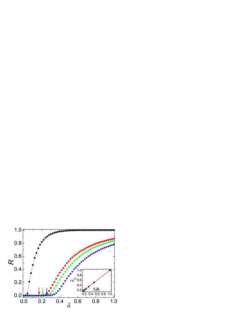
Figure 1: (color online) $R(\infty)$ as a function of the effective spreading rate $\lambda$ on BA networks with $\langle k\rangle=12$, $N=2000$. The black line represents the case of standard SIR model, and the blue, green and red curves represent the present model with $A=4$, 5 and 6, respectively. The arrows point at the critical points obtained from simulations. One can see clear from the inset that the analytic results agree well with the simulations.

III Simulation and results

Toward the standard SIR model, Moreno et al. obtained the analytical value of threshold $\langle k\rangle/\langle k^{2}\rangle$ Moreno2002 . Similarly, we consider the time evolution of $I_{k}(t)$, $S_{k}(t)$ and $R_{k}(t)$, which are the densities of infected, susceptible, and recovered nodes of degree $k$ at time $t$, respectively. Clearly, these variables obey the normalization condition:

$$I_{k}(t)+S_{k}(t)+R_{k}(t)=1.$$ (3)

Global quantities such as the epidemic prevalence are therefore expressed by the average over the various connectivity classes; $i.e.$, $R(t)=\sum_{k}P(k)R_{k}(t)$. Using the mean-field approximation, the rate equations for the partial densities in a network characterized by the degree distribution $P(k)$ can be written as:

$$\frac{dI_{k}(t)}{dt}=-I_{k}(t)+\lambda kS_{k}(t)\sum_{k^{\prime}}\frac{P(k^{\prime}|k)I_{k^{\prime}}(t)A}{k^{\prime}},$$ (4)

$$\frac{dS_{k}(t)}{dt}=-\lambda kS_{k}(t)\sum_{k^{\prime}}\frac{P(k^{\prime}|k)I_{k^{\prime}}(t)A}{k^{\prime}},$$ (5)

$$\frac{dR_{k}(t)}{dt}=I_{k}(t),$$ (6)

where the conditional probability $P(k^{\prime}|k)$ denotes the degree correlations that a vertex of degree $k$ is connected to a vertex of degree $k^{\prime}$. Considering the uncorrelated network, $P(k^{\prime}|k)=k^{\prime}P(k^{\prime})/\langle k\rangle$, thus Eq. (4) takes the form:

$$\frac{dI_{k}(t)}{dt}=-I_{k}(t)+\frac{\lambda k}{\langle k\rangle}S_{k}(t)\sum_{k}AP(k)I_{k}(t).$$ (7)

The equations (4-6), combined with the initial conditions $R_{k}(t)=0$, $I_{k}(0)=I_{k}^{0}$, and $S_{k}(0)=1-I_{k}^{0}$, completely define the SIR model on any complex network with degree distribution $P(k)$. We will consider in particular the case of a homogeneous initial distribution of infected nodes, $I_{k}^{0}=I^{0}$. In this case, in the limit $I^{0}\rightarrow 0$, we can substitute $I_{k}(0)\simeq 0$ and $S_{k}(0)=1$. Under this approximation and by taking the similar converting like from Eq. (4) to Eq. (7), Eq. (5) can be directly integrated, yielding

$$S_{k}(t)=e^{-\lambda k\phi(t)}.$$ (8)

where the auxiliary function $\phi(t)$ is defined as:

$$\phi(t)=\int_{0}^{t}\frac{\sum_{k}AP(k)I_{k}(t)}{\langle k\rangle}=\frac{\sum_{k}AP(k)R_{k}(t)}{\langle k\rangle}.$$ (9)

Focusing on the time evolution $\phi(t)$, one has

$$\frac{d\phi(t)}{dt} = \frac{\sum_{k}AP(k)I_{k}(t)}{\langle k\rangle}$$ (10)

$$= \frac{\sum_{k}AP(k)(1-R_{k}(t)-S_{k}(t))}{\langle k\rangle}$$ (11)

$$= \frac{A}{\langle k\rangle}-\phi(t)-\frac{\sum_{k}AP(k)S_{k}(t)}{\langle k\rangle}$$ (12)

$$= \frac{A}{\langle k\rangle}-\phi(t)-\frac{\sum_{k}AP(k)e^{-\lambda k\phi(t)}}{\langle k\rangle}.$$ (13)

Since $I_{k}(\infty)=0$ and consequently $\lim_{t\rightarrow\infty}{d\phi(t)}/{dt}=0$, we obtain from Eq. (13) the following self-consistent equation for $\phi_{\infty}$ as

$$\phi_{\infty}=\frac{A}{\langle k\rangle}(1-\sum_{k}P(k)e^{-\lambda k\phi_{\infty}}).$$ (14)

The value $\phi_{\infty}=0$ is always a solution. In order to have a non-zero solution, the condition

$$\frac{A}{\langle k\rangle}\frac{d(1-\sum_{k}P(k)e^{-\lambda k\phi_{\infty}})}{d\phi_{\infty}}\mid_{\phi_{\infty}=0}>1$$ (15)

must be fulfilled, which leads to

$$\frac{A\lambda}{\langle k\rangle}\sum_{k}kP(k)=\lambda A>1.$$ (16)

This inequality defines the epidemic threshold

$$\lambda_{c}=\frac{1}{A},$$ (17)

below which the epidemic prevalence is null, and above which it attains a finite value. Correspondingly, the previous works about epidemic spreading in SF networks present us with completely new epidemic propagation scenarios that a highly heterogeneous structure will lead to the absence of any epidemic threshold. While, now, it is $1/A$ instead (see the simulation and analytic results in Fig. 1). Furthermore, we can also find that the larger of identical infectivity $A$, the higher of density of $R(\infty)$ for the same $\lambda$ from Fig. 1.

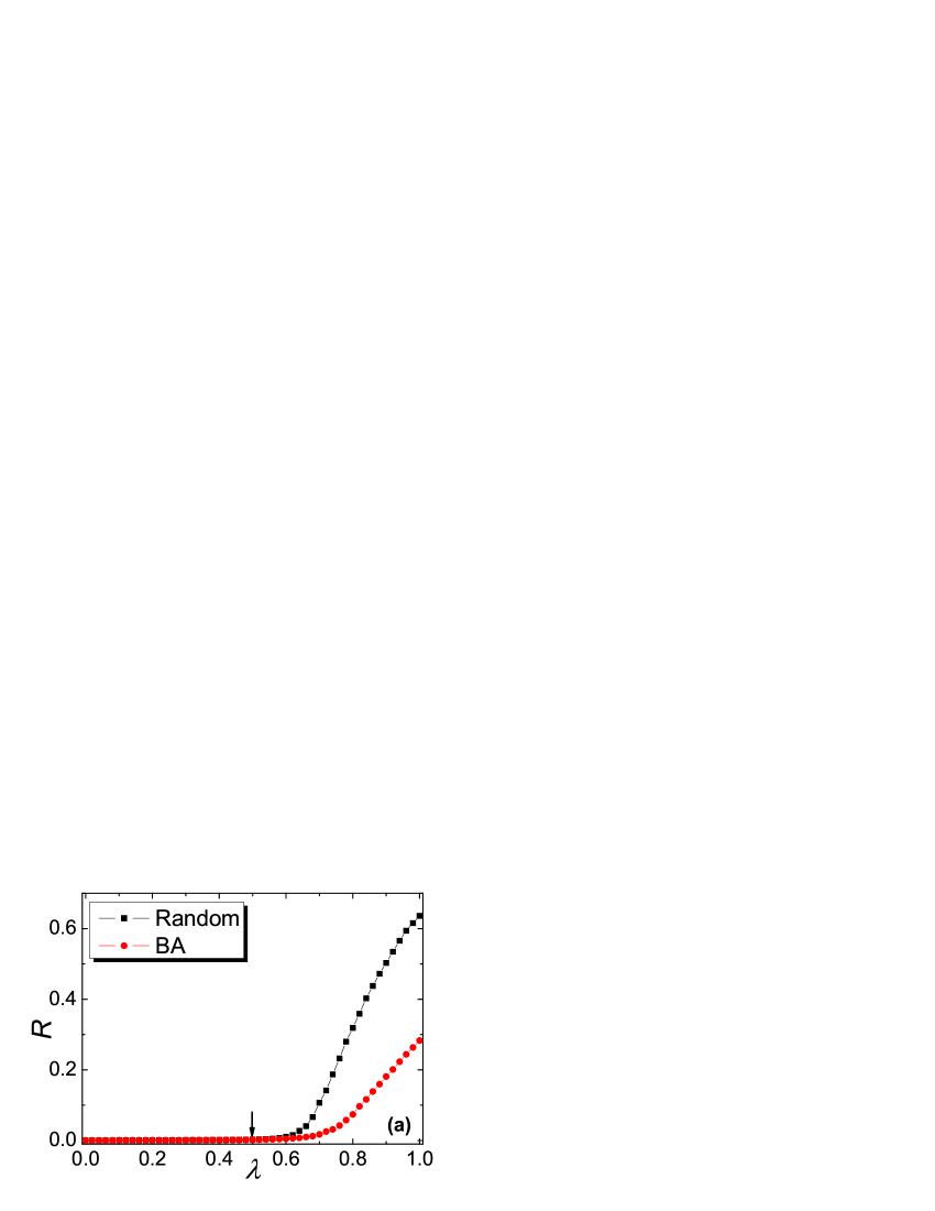
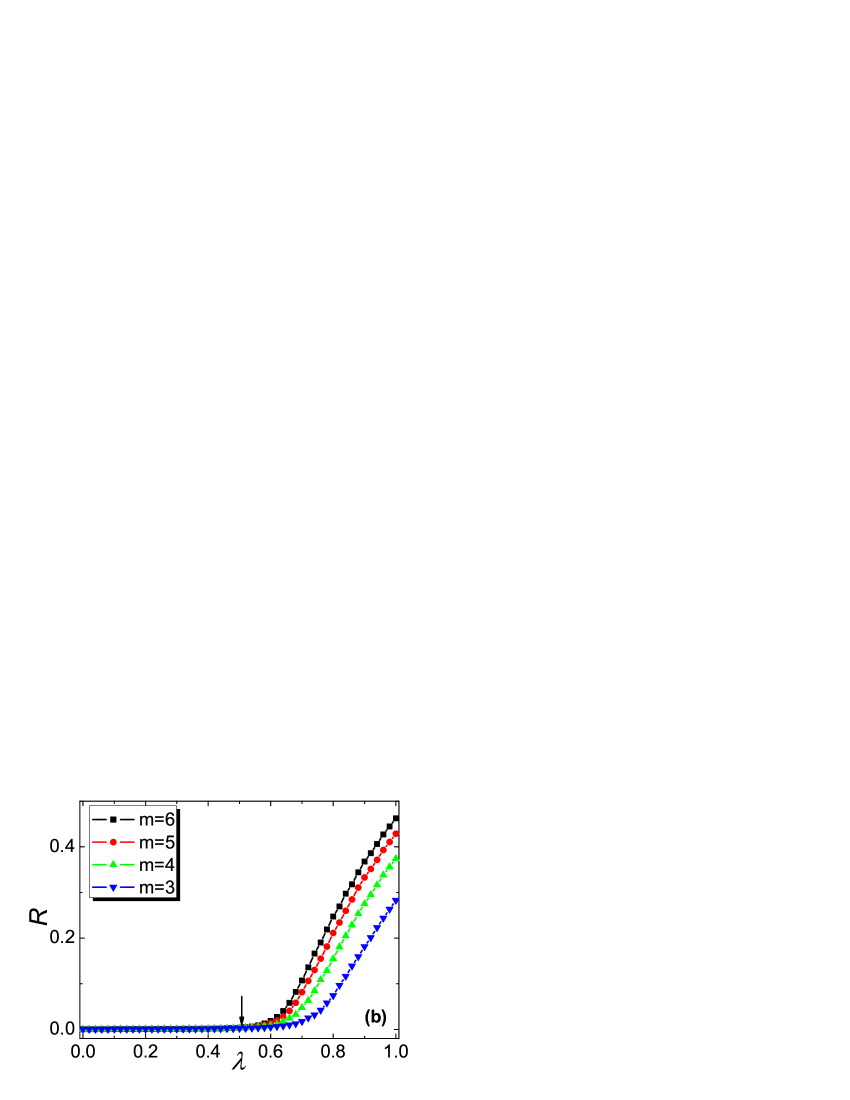
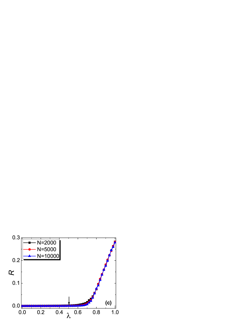
Figure 2: (color online) $R(\infty)$ as a function of the effective spreading rate $\lambda$ on BA and random networks with $\langle k\rangle=6$ (a), BA networks for different attachment number $m$ ($m=\langle k\rangle/2$) (b), and BA networks with different size $N$ (c). In figure (a) and (b), the network size is $N=2000$, and in all the above three plots, the infectivity is $A=2$.

From the analytical result, $\lambda_{c}=1/A$, one can see that the threshold value is independent of the topology if the underlying network is valid for the mean-field approximation ex . To further demonstrate this proposition, we next compare the simulation results on different networks. From Fig. 2, one can find that the threshold values of random networks, BA networks with different average degrees, and BA networks with different sizes are the same, which strongly support the above analysis. Note that, in the standard SIR model, there exists obviously finite-size effect May2001 ; Pastor2002 , while in the present model, there is no observed finite-size effect (see Fig. 3(c)).

IV Velocity and hierarchical spread

For further understanding the spreading dynamics of the present model, we study the time behavior of the epidemic propagation. Originated from the Eq. (8), $S_{k}(t)=e^{-\lambda k\phi(t)}$, which result is valid for any value of the degree of $k$ and the function $\phi(t)$ is positive and monotonically increasing. This last fact implies that $S_{k}$ is decreasing monotonically towards zero as time goes on. For any two values $k>k^{\prime}$, and whatever the initial conditions $S_{k}^{0}$ and $S_{k^{\prime}}^{0}$ are, there exists a time $t^{\prime}$ after which $S_{k}(t)<S_{k^{\prime}}{(t)}$. A more precise characterization of the epidemic diffusion through the network can be achieved by studying some convenient quantities in numerical spreading experiments in BA networks. First, we measure the average degree of newly recovered nodes at time $t$, which is equal to the average degree of newly infected nodes at time $t-1$,

$$\langle k_{R}{(t)}\rangle = \frac{\sum_{k}{k[R_{k}(t)-R_{k}(t-1)]}}{R(t)-R(t-1)}$$ (18)

$$= \frac{\sum{{}_{k}}{kI_{k}(t-1)}}{I(t-1)}$$ (19)

$$= \langle k_{inf}{(t-1)}\rangle.$$ (20)

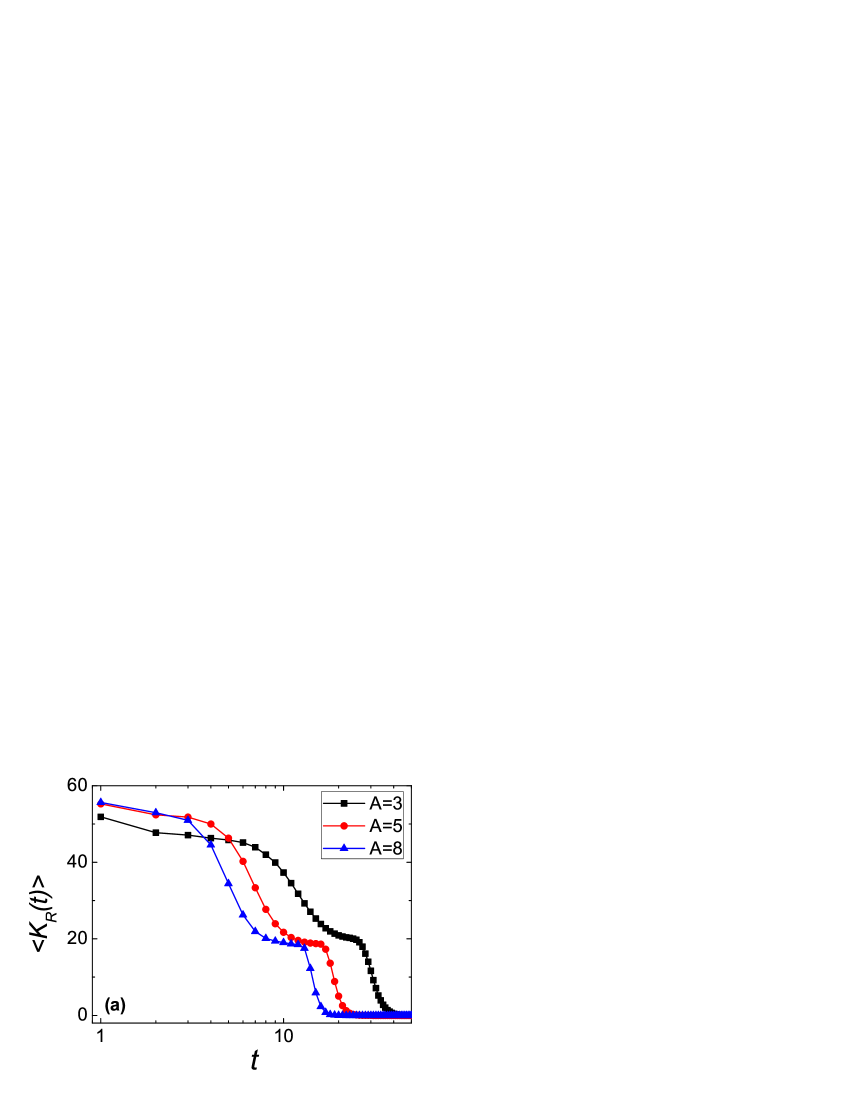
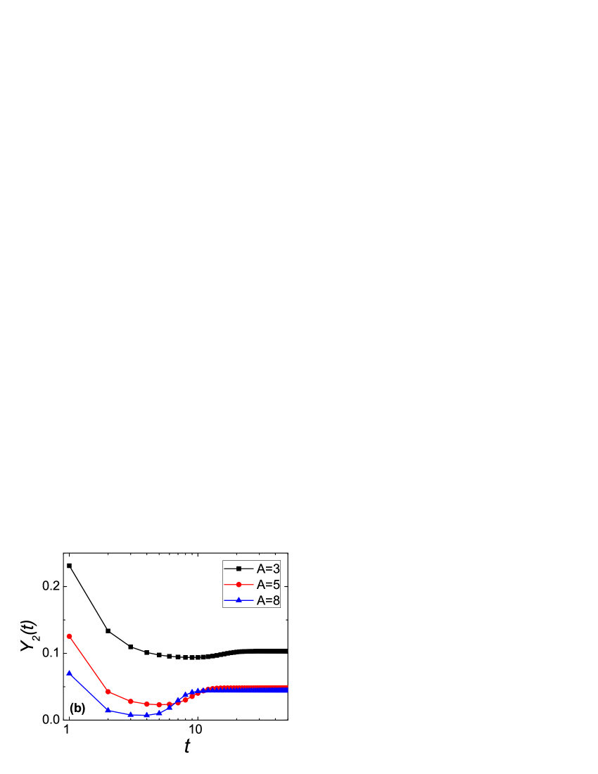
Figure 3: (color online) Time behavior of the average degree of the newly recovered nodes (a) and inverse participation ratio $Y_{2}$ (b) in BA networks of size $N=5000$.

In Fig. 3(a), we plot this quantity for BA networks as a function of the time $t$ for different values of $A$ and find a hierarchical dynamics with three plateaus. We can find that all of the curves show an initial plateau (see also a few previous works on hierarchical dynamics of the epidemic spreading M1 ; Barthelemy2005 ; Yan2005 ), which denotes that the infection takes control of the large degree vertices firstly. Once the highly connected hubs are reached, the infection pervades almost the whole network via a hierarchical cascade across smaller degree classes. Thus, $\langle k_{R}{(t)}\rangle$ decreases to a temporary plateau, which approximates $\langle k\rangle=2m$. At last, since the previously infected nodes recovered, all of which can be regarded as the barriers of spreading, the infection can only propagate to the smallest degree class. Then, the spreading process stops fleetly once the infected nodes are all recovered, as illustrated that $\langle k_{R}{(t)}\rangle$ decreases to zero rapidly.

Furthermore, we present the inverse participation ratio $Y_{2}(t)$ 21 to indicate the detailed information on the infection propagation. First we define the weight of recovered individuals with degree $k$ by $w_{k}(t)=R_{k}(t)/R(t)$. The quantity $Y_{2}(t)$ is then defined as:

$$Y_{2}(t)=\sum_{k}{w_{k}^{2}(t)}.$$ (21)

Clearly, if $Y_{2}$ is small, the infected individuals are homogeneously distributed among all degree classes; on the contrary, if $Y_{2}$ is relatively larger, then the infection is localized on some specific degree classes. As shown in Fig. 3(b), the function $Y_{2}(t)$ has a maximum at the early time stage, which implies that the infection is localized on the large degree $k$ classes, as can also inferred from Fig. 3(a). Afterwards $Y_{2}(t)$ decreases, with the infection progressively invading the lower degree classes, and providing a more homogeneous diffusion of infected vertices in the various degree classes. And then, $Y_{2}(t)$ increases gradually, which denotes the capillary invasion of the lowest degree classes. Finally, when $Y_{2}(t)$ slowly comes to the steady stage, the whole process ends.

V Conclusion

In this paper, we investigated the behaviors of SIR epidemics with an identical infectivity $A$. In the standard SIR model, the capability of the infection totally relies on the node’s degree, and therefore it leaves some practical spreading behaviors alone, such as in the pear-to-pear, sexual contact, Gmail server system, and marketing networks. Accordingly, this work is of not only theoretic interesting, but also practical value. We obtained the analytical result of the threshold value $\lambda_{c}=1/A$, which agree well with the numerical simulation. In addition, even though the activity of hub nodes are depressed in the present model, the hierarchical behavior of epidemic spreading is clearly observed, which is in accordance with some real situations. For example, in the spreading of HIV in Africa Bai2006 , the high-risk population, such as druggers and homosexual men, are always firstly infected. And then, this disease diffuse to the general population.

- (1) A. -L. Barabási and R. Albert, Science 286, 509 (1999).
- (2) R. Albert, and A. -L. Barabási, Rev. Mod. Phys. 74, 47 (2002).
- (3) R. Pastor-Satorras, and A. Vespignani, Epidemics and immunization in scale-free networks. In: S. Bornholdt, and H. G. Schuster (eds.) Handbook of Graph and Networks, Wiley-VCH, Berlin, 2003.
- (4) T. Zhou, Z. -Q. Fu, and B. -H. Wang, Prog. Nat. Sci. 16, 452 (2006).
- (5) F. Liljeros, C. R. Rdling, L. A. N. Amaral, H. E. Stanley, and Y. Åberg, Nature 411, 907 (2001).
- (6) S. Gupta, R. M. Anderson, and R. M. May, AIDS 3, 807-817 (1989).
- (7) M. MOrris, AIDS 97: Year in Review 11, 209-216 (1997).
- (8) R. Pastor-Satorras, and A. Vespignani, Phys. Rev. Lett. 86, 3200 (2001).
- (9) R. Pastor-Satorras, and A. Vespignani, Phys. Rev. E 63, 066117 (2001).
- (10) R. M. May, and A. L. Lloyd, Phys. Rev. E 64, 066112 (2001).
- (11) Y. Moreno, R. Pastor-Satorras, and A. Vespignani, Eur. Phys. J. B 26, 521 (2002).
- (12) M. Barthélemy, A. Barrat, R. Pastor-Satorras, and A. Vespihnani, Phy. Rev. Lett. 92, 178701 (2004).
- (13) T. Zhou, G. Yan, and B. -H. Wang, Phys. Rev. E 71, 046141 (2005).
- (14) A. Vázquez, Phys. Rev. Lett. 96, 038702 (2006).
- (15) M. A. Jovanovic, Modeling large-scale peer-to-peer networks and a case study of Gnutell [M.S. Thesis], University of Cincinnati, 2001.
- (16) Http://www.gnutella.com/.
- (17) T. Zhou, J. -G. Liu, W. -J. Bai, G. Chen, and B. -H. Wang, arXiv: physics/0604083 (Phys. Rev. E In Press).
- (18) Http://mail.google.com/mail/help/intl/en/about.html.
- (19) B. J. Kim, T. Jun, J. Y. Kim, and M. Y. Choi, Physica A 360, 493 (2005).
- (20) Note that, if the connections of the underlying networks are localized (e.g. lattices), then the mean-field approximation is incorrect and the threshold value is not equal to .
- (21) R. Pastor-Satorras, and A. Vespignani, Phys. Rev. E 65, 035108 (2002).
- (22) M. Barthélemy, A. Barrat, R. Pastor-Satorras, and A. Vespignani, J. Theor. Biol. 235, 275 (2005).
- (23) G. Yan, T. Zhou, J. Wang, Z. -Q. Fu, and B. -H. Wang, Chin. Phys. Lett. 22, 510 (2005).
- (24) B. Derrida and H. Flyvbjerg, J. Phys. A 20, 5273 (1987).
- (25) W. -J. Bai, T. Zhou, and B. -H. Wang, arXiv: physics/0602173.