Correlation Structures of Correlated Binomial Models and Implied Default Distribution

Abstract

We show how to analyze and interpret the correlation structures, the conditional expectation values and correlation coefficients of exchangeable Bernoulli random variables. We study implied default distributions for the iTraxx-CJ tranches and some popular probabilistic models, including the Gaussian copula model, Beta binomial distribution model and long-range Ising model. We interpret the differences in their profiles in terms of the correlation structures. The implied default distribution has singular correlation structures, reflecting the credit market implications. We point out two possible origins of the singular behavior.

1 Introduction

Describing and understanding crises in markets are intriguing subjects in financial engineering and econophysics [1, 2, 3, 4, 5, 6]. In the context of econophysics, the mechanism of systemic failure in banking has been studied [7, 8]. The Power law distribution of avalanches and several scaling laws in the context of the percolation theory were found. In addition, the network structures of real companies have been studied recently and their nonhomogeneity nature have been clarified [9, 10, 11]. This feature should be taken into account in the modeling of the dependent defaults of companies.

In financial engineering, many products have been invented to hedge the credit risks. CDS is a single-name credit derivative which is targeted on the default of one single obligor. Collateralized debt obligations (CDOs) are financial innovations to securitize portfolios of defaultable assets, which are called credit portfolios. They provide protections against a subset of total loss on a credit portfolio in exchange for payments. From an econophysical viewpoint, they give valuable insights into the market implications on default dependencies and the clustering of defaults. This aspect is very important, because the main difficulty in the understanding of credit events is that we have no sufficient information about them. By empirical studies of the historical data on credit events, the default probability $p_{d}$ and default correlation $\rho_{d}$ were estimated [12]. However, more detailed information is necessary in the pricing of credit derivatives and in the evaluation of models in econophysics. The quotes of the CDOs depend on the profiles of the default probability function [13]. This means that it is possible to infer the default loss probability function from market quotes. Recently, such an “implied” loss distribution function has attracted much attention in the studies of credit derivatives. Instead of using popular probabilistic models, implied loss distribution are proposed to use [14, 15].

In this paper, we show how to get detailed information contained in probability functions for multiple defaults. We compare the implied loss probability function with some popular probabilistic models and show their differences in terms of the correlation structure. The paper is organized as follows. In §2 we start from the definition of exchangeable Bernoulli random variables and explain the term “correlation structures”, the conditional expectation values and correlations. We introduce several notations of related quantities. Using the recursive relations, we show how to estimate them. We also point out that the method can be applied to any probability function of Bernoulli random variables, that are not necessarily exchangeable. In §3, we show how to infer the loss probability function for multiple defaults from the CDO market quotes by the entropy maximum principle. We compare the implied loss probability function with those of some popular probabilistic models in §4. The differences become strongly apparent in the behavior of the conditional correlations. The singular behavior of the implied loss function should be attributed to the nonlinear nature of multiple defaults or network structures of companies. We also try to read the credit market implications contained in the market quotes of CDOs and make a comment on “Correlation Smile”. Section 5 is devoted to the summary and future problems. In the appendix, we explain the relation between the profiles of probability functions and the correlation structures.

2 Calibration of Correlation Structures

In this section, we show a method of obtaining the “correlation structure” from the probability function. We denote the i-th asset’s (or obligor’s) state by Bernoulli random variable $X_{i}=0,1\hskip 5.69046pt(i=1,\cdots,N)$. If the asset is defaulted (or non-defaulted), $X_{i}$ takes $1(\mbox{resp.}0)$. We assume that $X_{i}$s are exchangeable. The exchangeability means that the joint probability function of $X_{i}$s is independent of any permutation of the values of $X_{i}$s. Denoting the joint probability function as

$$\mbox{Prob.}(X_{1}=x_{1},X_{2}=x_{2},\cdots,X_{N}=x_{N})=P(x_{1},x_{2},\cdots,x_{N}),$$

the next relation holds for any permutation $i_{1},i_{2},\cdots,i_{N}$ of $1,2,\cdots,N$,

$$P(x_{1},x_{2},\cdots,x_{N})=P(x_{i_{1}},x_{i_{2}},\cdots,x_{i_{N}}).$$

By assumption, the remaining degree of freedom in the joint probability function reduces to $N$. The joint probability for $i$ defaults and $j$ nondefaults only depends only on $i$ and $j$, and we denote it as $X_{i,j}$. The probability function for $n$ defaults $P_{N}(n)$ is written as

$$P_{N}(n)={}_{N}C_{n}\cdot X_{n,N-n}.$$

Here ${}_{N}C_{n}$ is the binomial coefficients.

The term “correlation structure” means the conditional expectation values $p_{i,j}$ and correlations $\rho_{i,j}$ . The subscript _i,j of $p_{i,j}$ and $\rho_{i,j}$ means that they are estimated under the condition that any $i$ (resp.$j$) of $N$ variables tale 1 (resp. 0). We also introduce $q_{i,j}$ as $1-p_{i,j}$. $p_{0,0}$ is the unconditional expectation value and it is nothing but the default probability $p_{d}$. $\rho_{0,0}$ is the unconditional default correlation $\rho_{d}$. More detailed explanations about $p_{i,j}$ and $\rho_{i,j}$ are given in the appendix. These quantities satisfy the following relations [16]

$$p_{i+1,j} = p_{i,j}+(1-p_{i,j})\rho_{i,j},$$ (1)

$$q_{i,j+1} = q_{i,j}+(1-q_{i,j})\rho_{i,j},$$ (2)

$$p_{i-1j}-p_{i,j-1} = -(1-p_{i-1j})\rho_{i-1j}-p_{i,j-1}\rho_{i,j-1}.$$ (3)

Figure 1: Solving process for $p_{i,j},q_{i,j}$ and $\rho_{i,j}$ from $X_{n.N-n}$.

Using these recursive relations, it is possible to estimate $p_{i,j}$ and $\rho_{i,j}$ from $P_{N}(n)$ or $X_{n,N-n}$. $X_{n,N-n}$ are on the bottom line of the Pascal triangle (See Fig.1). Then recursively solving the above eqs. (1)-(3) to the top vertex $(0,0)$ of the Pascal triangle, we obtain all $p_{i,j}$s and $\rho_{i,j}$s. For example, to obtain $p_{N-1,0}$ we use the relations

$$X_{N,0}=X_{N-1,0}\cdot p_{N-1,0}\hskip 8.5359pt\mbox{and}\hskip 8.5359ptX_{N-1,1}=X_{N-1,0}\cdot(1-p_{N-1,0}).$$ (4)

Solving for $p_{N-1,1}$, we get

$$p_{N-1,0}=\frac{X_{N,0}}{X_{N,0}+X_{N-1,1}}.$$ (5)

Likewise, we can estimate $p_{i,j}$ for general $i,j\leq N-1$. From $p_{i,j}$, $\rho_{i,j}$ are obtained by solving eq. (1).

The important point is that it is possible to estimate the correlation structure for any $P_{N}(n)$. In addition to theoretical models, empirically obtained probability functions can be studied. If $X_{i}$s are exchangeable, the obtained $p_{i,j}$ and $\rho_{i,j}$ are the ones defined in the text. In network terminology, the exchangeable case corresponds to the complete graph $K_{N}$ where all nodes are similar to each other with the same strength. If the network structure is not uniform, $X_{i}$s are not exchangeable. Even in such a case, the above method is applicable and gives many insights into the system. For example, if the network structure is treelike, the obtained correlation structure should be completely different from that in the exchangeable case. Its singular behavior strongly suggests the nonuniform network structure of the system.

3 Implied Default Distribution

We show how to infer the loss probability function based on market quotes of CDOs [14, 15]. In advance, we briefly explain CDOs. CDOs provide protection against losses in credit portfolios. Here “credit” means that the constituent assets of the portfolio can be defaulted. If an asset is defaulted, the portfolio loses its value. The interesting point of CDOs is that they are divided into several parts (called ’tranches’). Tranches have priorities that are defined by the attachment point $a_{L}$ and the detachment point $a_{H}$. The seller of protection agrees to cover all losses between $a_{L}K_{Total}$ and $a_{H}K_{Total}$, where $K_{Total}$ is the initial total notional of the portfolio. That is, if the loss is below $a_{L}K_{Total}$, the tranche does not cover it. The tranche begins to cover it Only when it exceeds $a_{L}K_{Total}$. If it exceeds $a_{H}K_{Total}$, the notional becomes zero. The seller of protection receives payments at a rate $s$ on the initial notional $(a_{H}-a_{L})K_{Total}$. Each loss that is covered reduces the notional on which payments are based. A typical CDO has a life of 5 years during which the seller of protection receives periodic payments. Usually these payments are made quarterly in arrears. In addition, to bring periodic payments up to date, an accrual payment is performed. Furthermore, the seller of protection makes a payment equal to the loss to the buyer of protection. The loss is the reduction in the notional principal times one less the recovery rate $R$.

iTraxx-CJ is an equally weighted portfolio of fifty CDSs on Japanese companies. The notional principal of CDSs is $K$ and $K_{Total}$ is $50\hskip 2.84544ptK$. The recovery rate is $R=0.35$. The standard attachment and detachment points are $\{0\%,3\%\}$,$\{3\%,6\%\}$,$\{6\%,9\%\}$,$\{9\%,12\%\}$ and $\{12\%,22\%\}$. We denote them as $\{a_{L}^{i},a_{H}^{i}\}$ with $i=1,\cdots,5$. Table 1 shows the tranche structures and quotes for iTraxx-CJ (Series 2) on August 30, 2005. We denote the upfront payment as $U_{i}$ and the annual payment rate as $s_{i}$ in basis points per year for the $i$th tranche. In the last row, we show the data for the index that cover all losses for the portfolio. In the 6th column, we show the initial notional $N_{0}^{i}$ in units of $K$.

Table 1: Quotes for iTraxx-CJ (Series 2) on August 30, 2005. Quotes are in basis points. Source: Tranche, Morgan Stanley Japan Securities Co. and Index, Bloomberg

Tranche	$a_{L}^{i}$	$a_{H}^{i}$	$s_{i}$[bps]	$U_{i}$[bps]	$N_{0}^{i}$	$N_{T,Implied}^{i}$
1	0%	3%	300	1313.3	1.5	1.1066
2	3%	6%	89.167	0	1.5	1.4361
3	6%	9%	28.5	0	1.5	1.4792
4	9%	12%	20.0	0	1.5	1.4854
5	12%	22%	14.0	0	5.0	4.9660
6	0%	100%	22.08	0	50	49.464

The value of contract is the present value of the expected cash flows. For simplicity, we treat 5 years as one term and write $T=5[year]$. We also assume that defaults occur in the middle of the period. We denote the notional principal for the $i$th tranche outstanding at maturity as $N_{T}^{i}$. The expected payoff of contract is

$$U_{i}N_{0}^{i}+T<N_{T}^{i}>s_{i}e^{-rT}+(N_{0}^{i}-<N_{T}^{i}>)\frac{s_{i}T}{2}e^{-r\frac{T}{2}}.$$ (6)

Here, $<A>$ means the expectation value of $A$ and $r$ is the risk-free rate of interest. The expected loss due to default is

$$(N_{0}^{i}-<N_{T}^{i}>)e^{-r\frac{T}{2}}.$$ (7)

The total value of the contract to the seller of protection is given by eqs. (6)-(7). Risk neutral values of $s_{i}$ and $U_{i}$ are determined so that eq. (6) equals eq. (7). Conversely, the market quotes for $s_{i}$ and $U_{i}$ tell us about the expected notional principal $<N_{T}^{i}>$. We write them as $N_{T,Implied}^{i}$. The last column in Table 1 shows them from the market quotes $s_{i}$ and $U_{i}$.

$N_{T}^{i}$ are random variables and are related to the number of defaults $n$ at maturity as

$$N_{T}^{i}(n)=\left\{\begin{array}[]{cc}N_{0}^{i}&n<\lceil\frac{a_{L}^{i}N}{1-R}\rceil\\ a_{H}N-n(1-R)&\lceil\frac{a_{L}^{i}N}{1-R}\rceil\leq n<\lceil\frac{a_{H}^{i}N}{1-R}\rceil\\ 0&n\geq\lceil\frac{a_{H}^{i}N}{1-R}\rceil.\\ \end{array}\right.$$ (8)

Here, $\lceil x\rceil$ means the smallest integer greater than $x$. To calculate the expectation value of $N_{T}^{i}(n)$, the default probability function $P_{N}(n)$ is necessary. Inversely, using the data on these expectation values $N_{T,Implied}^{i}$, we try to infer $P_{N}(n)$ from the maximum entropy principle. It states that one should consider the model $P_{N}(n)$ that maximizes the entropy functional subject to the conditions imposed by previous known information.

The entropy functional $S[P_{N}(n)]$ is defined as

$$S[P_{N}(n)]=\sum_{n=0}^{N}{}_{N}C_{n}\cdot X_{n,N-n}\log X_{n,N-n}$$ (9)

$$+ \sum_{i=1}^{6}\lambda^{i}(\sum_{n=0}^{N}{}_{N}C_{n}\cdot X_{n,N-n}N_{T}^{i}(n)-N_{T,Implied}^{i}).$$

In order to impose the condition $<N_{T}^{i}>=N_{T,Implied}^{i}$ on $P_{N}(n)$, we introduce six Lagrange multipliers $\lambda^{i}$. By maximizing 9, we get the implied joint probability $X_{n,N-n}$ as

$$X_{n,N-n}\propto\left\{\begin{array}[]{cc}e^{-\lambda_{6}n-\lambda^{1}(a_{H}^{1}N-n(1-R))}\prod_{i=2}^{5}C_{i}&n<n_{H}^{1}\\ e^{-\lambda_{6}n-\lambda^{j+1}(a_{H}^{j+1}N-n(1-R))}\prod_{i=j+2}^{5}C_{i}&n_{H}^{j}\leq n<n_{H}^{j+1}\\ e^{-\lambda_{6}n}&n\geq n_{H}^{5}.\\ \end{array}\right.$$ (13)

Here, we use the notation $n_{H}^{i}=\lceil\frac{a_{H}^{i}N}{1-R}\rceil$ and $C_{i}=\exp(-\lambda^{i}N^{i}_{T}(n))$.

Figure 2: Plot of implied default distribution for fifty Japanese companies on August 30, 2005.

The six Lagrange multiplier were calibrated so that the condition $<N_{T}^{i}>=N_{T,Implied}^{i}$ is satisfied. We use the simulated annealing method and fix these parameters. Figure 2 shows the result of fitting eq. (13) to iTraxx-CJ data on August 30, 2005. About the convergence, it is satisfactory and all premiums are recovered within $1\%$. From the inset figure, which shows a semilog plot of the distribution, we see a hunchy structure or a second peak. $P_{N}(n)$ decreases monotonically up to the fourth tranche ($n\leq 9$), then $P_{N}(n)$ begins to increase. In the fifth tranche $n_{H}^{4}=10<n\leq n_{H}^{5}=17$, $P_{N}(n)$ has a peak and then decreases to zero. We also see some joints between tranches at $n_{H}^{j}$. The latter is an artifact of the maximum entropy principle.

4 Comparison with Popular Probabilistic Models

In this section, we compare the behaviors of the loss probability function $P_{N}(n)$ of some popular probabilistic models with the implied loss distribution function from the viewpoint of the correlation structure. In particular, we focus on $\rho_{i,0}$ and $p_{i,0}$. As probabilistic models, we consider the next three models. These models are defined by the mixing function $f(p)$ that express the joint probability function $X_{i,j}$ as [1, 16]

$$X_{i,j}=\int f(p^{\prime}){p^{\prime}}^{i}(1-p^{\prime})^{j}dp^{\prime}.$$ (14)

We choose the Gaussian copula (GC) model, which is a standard model in financial engineering [15], the beta binomial distribution (BBD), which is the benchmark model among exchangeable correlated binomial models [16] and the long-range Ising (LRI) model [5]. The reason for adopting LRI, instead of the Ising model on some lattice, is that in financial engineering all obligors are usually assumed to be related to each other with the same strength and that the network structure is uniform. In addition, the long-range Ising model can be expressed as a superposition of two binomial distributions for sufficiently large $N$ and it is very tractable.

1. Gaussian Copula (GC) Model.

   The model incorporates the default correlation $\rho_{d}$ by a common random factor $Y$ and an asset correlation $\rho_{a}$. If the factor $Y$ is fixed as $Y=y$, the variables $X_{i}$ become independent with the probability $\mbox{Prob.}(X_{i}=1)=p(y)$. The explicit form of the mixing function is

   $$f(p(y))=\Phi(\frac{K-\sqrt{\rho_{a}}y}{\sqrt{1-\rho_{a}}}).$$ (15)

   Here, $K=\Phi^{-1}(p_{d})$ with the normal cumulative function $\Phi(K)$ and $Y$ obeys the normal distribution $Y\sim N(0,1^{2})$. $X_{i,j}$ are then given as

   $$X_{i,j}=<p(y)^{i}(1-p(y))^{j}>_{Y}.$$ (16)

   $<\hskip 14.22636pt>_{Y}$ denotes the expectation value over the random variable $Y$. In order to estimate $\rho_{d}$, we use the relation $\rho_{d}=\frac{X_{2,0}-p_{d}^{2}}{p_{d}(1-p_{d})}$.

2. Beta Binomial Distribution (BBD) Model.

   The mixing function $f(p^{\prime})$ is the beta distribution.

   $$f(p^{\prime})=\frac{{p^{\prime}}^{\alpha-1}(1-p^{\prime})^{\beta-1}}{\mbox{B}(\alpha,\beta)}.$$ (17)

   Here $\mbox{B}(\alpha,\beta)$ is the beta function. $X_{i,j}$ are given as

   $$X_{i,j}=\frac{\mbox{B}(\alpha+i,\beta+j)}{\mbox{B}(\alpha,\beta)}.$$ (18)

   It is easy to show that $p_{0,0}=p_{d}=\frac{\alpha}{\alpha+\beta}$ and $\rho_{0,0}=\rho_{d}=\frac{1}{\alpha+\beta+1}$.

   We note that BBD is the benchmark model among exchangeable correlated binomial models. $\rho_{i,j}$ depend on $i,j$ through the form $i+j$ as $\rho_{i,j}=\frac{\rho_{d}}{1+(i+j)\rho_{d}}$. As the result, $p_{i,j}$ becomes a linear function of $i$ for the fixed $i+j=k$ as

   $$p_{i,j}=\frac{p_{d}(1-\rho_{d})+i\cdot\rho_{d}}{1+(k-1)\rho_{d}}.$$

   BBD is the “linear” model [16] that is why we call it the benchmark model. One can see the nonlinearity of other models by checking the differences of $\rho_{i,j}$ and $p_{i,j}$ from those of BBD.

3. Long-Range Ising (LRI) Model [17].

   The mixing function $f(p^{\prime})$ is the superposition of two $\delta$ functions $\delta(p^{\prime}-p)$ and $\delta(p^{\prime}-(1-p))$.

   $$f(p^{\prime})=(1-\alpha)\cdot\delta(p^{\prime}-p)+\alpha\delta(p^{\prime}+(1-p)).$$ (19)

   $X_{i,j}$ are given as

   $$X_{i,j}=(1-\alpha)p^{i}(1-p)^{j}+\alpha(1-p)^{i}p^{j}.$$ (20)

   It is easy to show that $p_{0,0}=p_{d}=(1-\alpha)p+\alpha(1-p)$ and $\rho_{0,0}=\rho_{d}=\frac{\alpha(1-\alpha)(2p-1)^{2}}{p_{d}(1-p_{d})}$.

Figure 3 shows a plot of the implied distribution of the previous section with the probability function $P_{N}(n)$ of the above three models. The models have three parameters : the number of variables $N$, the default probability $p_{d}$ and default correlation $\rho_{d}$. We set them with the same values of the implied distribution as $N=50$, $p_{d}=1.65\%$ and $\rho_{d}=6.55\%$. We see that all three models give poor fits to the implied distribution. GC and BBD show a monotonic dependence on $n$. The LRI model has a nonmonotonic dependence and has a hump at $n=N$.

Figure 3: Plot of implied default distribution (Fig.2) and the probability functions of popular pricing models. Implied distribution (solid), GC ($\times$), BBD ($+$) and LRI (dashed-dotted line). We set $N=50$,$p=1.65\%$ and $\rho_{d}=6.55\%$.

Next, we compare their correlation structures. Figure 4 depicts $\rho_{i,0}$ and $p_{i,0}$. $\rho_{i,0}$ for GC has a low peak and decays to zero slowly. BBD’s $\rho_{i,0}$ decays slowly as $\rho_{i,0}=\frac{\rho_{d}}{1+i\rho_{d}}$. On the other hand, LRI’s $\rho_{i,0}$ rapidly increases to $1$ and decays rapidly to zero. This behavior means that GC is weakly nonlinear and LRI is strongly nonlinear.

As for $p_{i,0}$, recall the relation $p_{i+1,0}=p_{i,0}+(1-p_{i,0})\rho_{i,0}$ (eq.( 1)). With the same $p_{d}$ and $\rho_{d}$, we have $p_{0,0}=p_{d}$ and $p_{1,0}=p_{d}+(1-p_{d})\rho_{d}$. All curves $(i,p_{i,0})$ go through the two points $(0,p_{d})$ and $(1,p_{d}+(1-p_{d})\rho_{d})$. As $\rho_{i,0}$ for $i\geq 1$ differs among the models and the implied one, the curves $(i,p_{i,0})$ depart from each other for $i\geq 2$. LRI’s $\rho_{i,0}$ rapidly increases to $1$. $p_{i,0}$ also increases to 1 rapidly. For $i=3$, $p_{i,0}\simeq 1$ and this means that all the obligors always default simultaneously if three of them are defaulted, which is the biggest avalanche. As the result, $P_{N}(n)$ has a hump in its tail $n=N$. GC’s $p_{i,0}$ and BBD’s $p_{i,0}$ increase to 1 with $i$ slowly. The distribution of the size of avalanches should be very wide and $P_{N}(n)$ comes to have a long tail.

Figure 4: Plots of $\rho_{i,0}$ and $p_{i,0}$ (inset figure).

The implied one’s $\rho_{i,0}$ has a medium peak at $i=1$ and then rapidly decreases to zero for $i\geq 5$. Comparing it with those of BBD, we see that the implied loss distribution function is nonlinear. Its behavior is completely different from those of both GC and BBD. $p_{i,0}$ increases rapidly with $i$ compared with GC and BBD and soon saturates to some maximum value $\simeq 0.35$ at $i=5$. The credit market expects that if more than 5 defaults occur, the obligors default almost independently. The size of an avalanche of simultaneous defaults is smaller than that of the Ising model. However, the probability that a medium-size of avalanche of defaults occurs is large compared with the GC and BBD.

Figure 5: Implied default distribution on August 30, 2005. iTraxx-CJ (in solid), iTraxx-Europe (dashed) and CDX IG (+).

We also studied the correlation structures of the implied loss functions of iTraxx-Europe and CDX IG (U.S.A.), which are CDOs of European and American companies ($N=125$) [15]. The implied distributions and $\rho_{i,0}$ are plotted in Fig. 5. The implied loss functions are more complex than that of iTraxx-CJ. $\rho_{i,0}$ shows the same singular behavior with those of iTraxx-CJ and the singular behavior seems to be a universal property.

About the origin of the singular behavior of $\rho_{i,0}$, we point out two possibilities. The first is that the probabilistic rule that governs the defaults of obligors is essentially new and nonlinear. The second is that the nonuniform network structure of the dependency relation of the obligors is reflected in $\rho_{i,0}$. If the network structure is not uniform, it affects the resulting correlation structure. As a result, $\rho_{i,0}$ looks singular compared with those of the models on the uniform network.

Table 2: Implied tranche correlations and entropy maximum correlation for 5-year iTraxx-CJ tranches on August 30, 2005.

$\{0\%,3\%\}$	$\{3\%,6\%\}$	$\{6\%,9\%\}$	$\{9\%,12\%\}$	$\{12\%,22\%\}$	Entropy
13.5%	1.20%	2.58%	4.95 %	9.71 %	6.55 %

At last we comment on the tranche (compound) correlation, which is the standard correlation measure in financial engineering [13]. The method suggests the correlation $\rho_{d}^{i}$ so that the expected loss equals the expected payoffs for the $i-$th tranche, it is called “tranche correlations”. The expected values are estimated with GC. Table 2 shows the tranche correlations for the quotes of iTraxx-CJ on August 30, 2005. In the last column, we show the maximum entropy value derived from the implied default distribution. As we showed previously, the GC gives a poor fit to the implied distribution. The tranche correlations are completely different from the entropy maximum value. In addition, it depends on which tranche the correlation is estimated. Such a dependence is known as a “correlation smile” [18]. We think that the “true” default correlation is approximately given by the maximum entropy value and that tranche correlations are an artifact of using GC to fit the market quotes. As long as the probabilistic model gives a poor fit to the market quotes, the default correlation varies among the tranches. This is the origin of the “correlation smile”.

5 Conclusions

We show how to estimate the conditional probabilities $p_{i,j}$ and correlations $\rho_{i,j}$ from $P_{N}(n)$. BBD is the benchmark model among exchangeable correlated binomial models and $\rho_{i,j}$ behave as $\rho_{i,j}=\frac{\rho_{d}}{1+(i+j)\rho_{d}}$. If the obtained $\rho_{i,j}$ depends on $i,j$, which is considerably different from those of BBD, there are two possibilities. The first one is that the probabilistic rule that governs $X_{i}$s is strongly nonlinear. The second one is that the assumption of the exchangeablity is wrong. The network structure of the dependency relation among $X_{i}$s is nonuniform.

We have inferred the loss probability function for multiple defaults based on the market quotes of CDOs and the maximum entropy principle. The profile is completely different from those of some popular probabilistic models, namely GC, BBD and LRI. $\rho_{i,0}$ has a medium peak and then rapidly decreases to zero for $i\geq 5$. The origin of the singular behavior can be attributed to the above two possibilities.

In order to clarify the mechanism of the singular behavior of $\rho_{i,0}$, it is necessary to study correlated binomial models on networks. In particular, the dependence of $\rho_{i,0}$ on the network structure should be understood. Recently, the authors have shown how to construct a linear correlated binomial model on networks in general [19]. By applying the method of the present paper to the model, it is possible to understand the relation between the network structure and the correlation structures. More detailed studies of real companies’ dependency structures have been performed recently [20]. Instead of the implied loss function, a real loss distribution function has been estimated. Promoting these studies, we think that it is possible to understand the dependency structure of multiple defaults and to propose a theoretical model of the pricing of CDOs.

Appendix A Probability Function and Correlation Structure

In this section, we explain the relation between $P_{N}(n)$ and the correlation structures $p_{i,j}$ and $\rho_{i,j}$. We introduce the products of $X_{i}$ and $1-X_{j}$, which exhaust all observables of the system.

$$\Pi_{i,j}=\prod_{i^{\prime}=1}^{i}X_{i^{\prime}}\prod_{j^{\prime}=i+1}^{i+j}(1-X_{j^{\prime}})$$ (21)

The following definitions are their unconditional and conditional expectation values (see Fig. 6.).

$$X_{i,j} = <\Pi_{i,j}>.$$ (22)

$$p_{i,j} = <X_{i+j+1}|\Pi_{i,j}=1>=<\Pi_{i+1,j}|\Pi_{i,j}>=\frac{X_{i+1,j}}{X_{i,j}}.$$ (23)

$$q_{i,j} = <1-X_{i+j+1}|\Pi_{i,j}=1>=<\Pi_{i,j+1}|\Pi_{i,j}>=\frac{X_{i,j+1}}{X_{i,j}}.$$ (24)

Here $<A|B>$ means the expectation value of the random variable $A$ under the condition that $B$ is satisfied. $X_{0,0}=1$, $X_{1,0}=p_{0,0}$ and $X_{0,1}=1-p_{0,0}=q_{0,0}$. All information of the model is contained in $X_{i,j}$. The joint probability $P(x_{1},x_{2},\cdots,x_{N})$ with $\sum_{i^{\prime}=1}^{N}x_{i^{\prime}}=n$ is given by $X_{n,N-n}$. The probability function $P_{N}(n)$ is given as

$$P_{N}(n)\equiv\mbox{Prob}(\sum_{i=1}^{N}X_{i}=n)={}_{N}C_{n}\cdot X_{n,N-n}.$$

Figure 6: Pascal’s triangle representation of $X_{i,j}$ up to $i+j\ \leq 2$ and $p_{i,j},q_{i,j}$ . $X_{0,0}=<1>$, $X_{1,0}=<X_{1}>=p$, $X_{0,1}=<1-X_{1}>=1-p=q$ etc.

We also introduce the conditional correlation

$$\mbox{Corr}(X_{i+j+1},X_{i+j+2}|\Pi_{i,j}=1)=\rho_{i,j}.$$ (25)

The correlation between $X_{i}$ and $X_{j}$ is defined as

$$\mbox{Corr}(X_{i},X_{j})\equiv\frac{<X_{i}X_{j}>-<X_{i}><X_{j}>}{\sqrt{<X_{i}>(1-<X_{i}>)<X_{j}>(1-<X_{j}>)}}.$$ (26)

Its conditional ones are defined by replacing expectation values with conditional expectation values.

The conditional quantities $p_{i,j},q_{i,j}$ and $\rho_{i,j}$ must obey the recursive relations from eqs. (1)-(3). The reason is that the following two relations must hold for the system to be consistent. The first one is $p_{i,j}+q_{i,j}=1$ for any $i,j$, because of the identity $<1|\Pi_{i,j}=1>=<X_{i+j+1}+(1-X_{i+j+1})|\Pi_{i,j}=1>=1$. The second one is the commutation relation

$$q_{i+1,j}\cdot p_{i,j}=p_{i,j+1}\cdot q_{i,j}=\frac{X_{i+1,j+1}}{X_{i,j}}.$$ (27)

These two relations are guaranteed to hold when $p_{i,j},q_{i,j}$ and $\rho_{i,j}$ satisfy the above consistency relations.

We explain the meaning of these quantities. The first one is $p_{0,0}$, the unconditional expectation value of $X_{i}$. Its meaning is clear and it is the probability that $X_{i}$ takes 1. In the context of a credit portfolio problem, it is the default probability $p_{d}$. It is easy to estimate it from $P_{N}(n)$ as

$$p_{d}=p_{0,0}=<X_{i}>=<n>/N.$$ (28)

The unconditional correlation $\rho_{0,0}$ is the default correlation $\rho_{d}$ in the credit risk context. It is also easy to estimate it as

$$\rho_{d}=\rho_{0,0}=\frac{<n^{2}-n>/N(N-1)-p_{d}^{2}}{p_{d}(1-p_{d})}.$$ (29)

Its estimation is important in the evaluation of the prices of credit derivatives. One reason is that it is related to the conditional default probability $p_{1,0}$ from eq. (1) as

$$p_{1,0}=p_{d}+(1-p_{d})\rho_{d}.$$ (30)

If one obligor is defaulted, the default probability $p_{d}$ changes to $p_{1,0}$. The second reason is that it gives the simultaneous default probability for $X_{i}$ and $X_{j}$ as

$$\mbox{Prob.}(X_{i}=1,X_{j}=1)=p_{d}^{2}+p_{d}(1-p_{d})\rho_{d}.$$ (31)

Usually, $p_{d}$ is small and the simultaneous default probability is mainly governed by the second term.

Regarding $p_{i,j}$ with $i\hskip 2.84544pt\mbox{or}\hskip 2.84544ptj>0$, we note one point. From the definition, $p_{i,j}$ means the default probability under the condition $\Pi_{i,j}=1$. $\rho_{i,j}$ also means the default correlation in the same situation. $p_{l,m}$ with $l\geq i$ and $m\geq j$ are closely related to the default probability function $P_{N-(i+j)}(n-(i+j)|\Pi_{i,j}=1)$. We write $k=i+j$ and the next relation holds for $n\geq k$.

$$P_{N-k}(n-k|\Pi_{i,j}=1)={}_{N-k}C_{n-k}\cdot<\prod_{l=1}^{n-k}X_{k+l}\prod_{m=1}^{N-n}(1-X_{n+m})|\Pi_{i,j}=1>$$ (32)

We evaluate the expectation value with $p_{l,m}$ and $q_{l,m}$, and we get

$$P_{N-k}(n-k|\Pi_{i,j}=1)={}_{N-k}C_{n-k}\cdot\prod_{l=0}^{n-k-1}p_{i+l,j}\prod_{m=0}^{N-n-1}q_{n-k+i,j+m}\hskip 8.5359ptn\geq k.$$ (33)

This relation indicates that the Pascal Triangle with the vertex $(i,j),(N-j,j)$, and $(i,N-i)$ contains all information for the case $\Pi_{i,j}=1$ (See Fig. 7). In order to know the loss probability function under the condition $\Pi_{i,j}=1$, we only need to know $p_{l,m}$ and $q_{l,m}$ in the restricted Pascal Triangle.

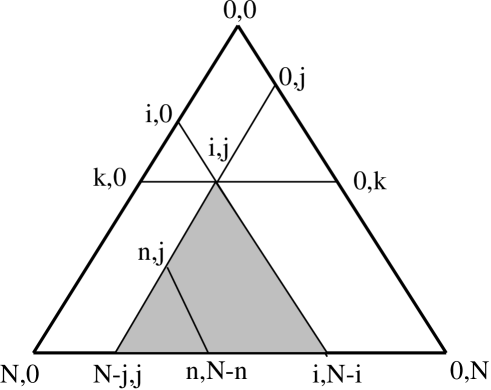
Figure 7: Restricted Pascal Triangle with the vertex $(i,j),(N-j,j)$ and $(i,N-i)$. $p_{l,m}$ and $\rho_{l,m}$ in the triangle govern the behavior of the system under the condition $\Pi_{i,j}=1$.

The $i$-dependence of $\rho_{i,0}$ and $p_{i,0}$ is closely related to the behavior of the probability function $P_{N}(n)$ for $n\geq i$. By the relation, we can understand the cascading structure of the simultaneous defaults. Hereafter, as we are interested in the credit risk problem, we assume that $p_{0,0}=p_{d}$ is small.

First, we note that $P_{N}(n)$ can be expressed in the following form for $n\geq i$.

$$P_{N}(n)=\frac{{}_{N}C_{n}}{{}_{N-i}C_{n-i}}\cdot X_{i,0}\cdot P_{N-i}(n-i|\Pi_{i,0}=1).$$ (34)

The derivation is based on the following relation.

$$P_{N-i}(n-i|\Pi_{i,0}=1)={}_{N-i}C_{n-i}\times<\prod_{l=i+1}^{n}X_{l}\prod_{m=n+1}^{N}(1-X_{m})|\Pi_{i,0}=1>$$ (35)

$$= {}_{N-i}C_{n-i}\times<\prod_{l=1}^{n}X_{l}\prod_{m=n+1}^{N}(1-X_{m})|\Pi_{i,0}=1>$$

$$= {}_{N-i}C_{n-i}\times<\prod_{l=1}^{n}X_{l}\prod_{m=n+1}^{N}(1-X_{m})>/<\prod_{l=1}^{i}X_{i}>$$

$$= {}_{N-i}C_{n-i}\times\frac{P_{N}(n)}{{}_{N}C_{n}}/X_{i,0}.$$

Equation (34) tells us about the behavior of $P_{N}(n)$ for $n\geq i$.

We classify the behavior $\rho_{i,0}$ into two cases.

1. Short-tail case :

   The probability function $P_{N}(n)$ develops a short tail in the case where $\rho_{i,0}$ rapidly decreases with $i$ and $\rho_{i,j}=0$ for $i\geq k$ and $j\leq i-k$ with $k<<N$. For the case $\Pi_{i,j}=0$ with $i\geq k$ and $j\leq i-k$, all variables become independent. $X_{i,j}$ is estimated as

   $$X_{i,j}=X_{k,0}\cdot<\Pi_{i,j}|\Pi_{k,0}=0>=X_{k,0}\cdot p_{k,0}^{i-k}\cdots q_{k,0}^{j}.$$

   The probability function $P_{N}(n)$ for $n\geq k$ becomes

   $$P_{N}(n)={}_{N}C_{n}\cdot\frac{X_{k,0}}{p_{k,0}^{k}}\cdot p_{k,0}^{n}\cdot q_{k,0}^{N-n}.$$

   $P_{N}(n)$ becomes proportional to the binomial distribution $\mbox{Bi}(N,p_{k,0})$ and has a short tail. It has a hump at $n\simeq N\cdot p_{k,0}$. In particular, if $p_{k,0}\simeq 1$, the probability function has a hump at $n=N$.

2. Long-tail case :

   The probability function has a long tail in the case where $\rho_{i,0}$ is small and gradually decreases with $i$. The random variables are weakly coupled. The $i$-dependence of $p_{i,0}$ is given by $p_{i+1,0}=p_{i,0}+(1-p_{i,0})\rho_{i,0}$ and $p_{i,0}$ gradually increases with $i$. If we assume $\rho_{i,0}=0$, $P_{N}(n)$ becomes proportional to the binomial distribution $\mbox{Bi}(N,p_{i,0})$ for $n\geq i$.

   $$P_{N}(n)={}_{N}C_{n}\cdot\frac{X_{i,0}}{p_{i,0}^{i}}\cdot p_{i,0}^{n}\cdot q_{i,0}^{N-n}\hskip 8.5359pt\mbox{for}\hskip 8.5359ptn\geq i.$$

   However, $\rho_{i,0}$ is not zero and $p_{i,0}$ gradually increases with $i$. For $n\geq i+1$, $P_{N}(n)$ behaves as

   $$P_{N}(n)={}_{N}C_{n}\cdot\frac{X_{i+1,0}}{p_{i+1,0}^{i}}\cdot p_{i+1,0}^{n}\cdot q_{i,0}^{N-n}\hskip 8.5359pt\mbox{for}\hskip 8.5359ptn\geq i.$$

   $X_{i+1,0}=X_{i,0}\cdot p_{i,0}$, we have

   $$P_{N}(n)={}_{N}C_{n}\cdot\frac{X_{i,0}}{p_{i+1,0}^{i}}\cdot\frac{p_{i,0}}{p_{i+1,0}}\cdot p_{i+1,0}^{n}\cdot q_{i,0}^{N-n}\hskip 8.5359pt\mbox{for}\hskip 8.5359ptn\geq i.$$

   As $p_{i+1,0}>p_{i,0}$, the overall scale $\frac{X_{i,0}}{p_{i+1,0}^{i}}\cdot\frac{p_{i,0}}{p_{i+1,0}}$ is smaller than $\frac{X_{i,0}}{p_{i,0}^{i}}$. Apart from the overall factor, $P_{N}(n)$ becomes proportional to $\mbox{Bi}(N,p_{i,0})$ with a larger $p_{i,0}$ for a larger $i$. Compared with that in the short-tail case, the decrease in $P_{N}(n)$ with $n$ is milder and $P_{N}(n)$ has a longer tail.

References

- [1] P. J. Schönbucher: Credit Derivatives Pricing Models: Model, Pricing and Implementation, U.S. John Wiley & Sons (2003).
- [2] J.-P. Bouchaud and M. Potters: Theory of Financial Risks, Cambridge University Press (2000).
- [3] R. A. Mantegna and H. E. Stanley; An Introduction to Econophysics, Cambridge University Press (2000).
- [4] M. Davis and V. Lo; Quantitative Finance 1 (1999) 382.
- [5] K. Kitsukawa, S. Mori, and M. Hisakado; Physica A368 (2006) 191.
- [6] A. Sakata, M. Hisakado and S. Mori; J.Phys.Soc.Jp. 76(2007) 054801.
- [7] A. Aleksiejuk and A. Holyst; Physica A299,(2001) 198.
- [8] G. Iori and S. Jaferey; Physica A299(2001) 205.
- [9] W. Souma, Y. Fujiwara, and H. Aoyama; Physica A324 (2003) 396.
- [10] A. M. Chmiel, J. Sienkiewicz, J. Suchecki and J.A. Holyst; Physica A383(2007) 134.
- [11] D. Helbing, S. Lammear, P. Seba, and T. Platkowski; Phys. Rev. E70 (2004) 066116.
- [12] N. J. Jobst and A. de Servigny; An Empirical Analysis of Equity Default Swaps (II): Multivariate insights, Working Paper, S&P (2005).
- [13] C. C. Finger; Issues in the Pricing of Synthetic CDOs, J. of Credit Risk, 1 (2005) 1.
- [14] L. Vacca; Unbiased risk-neutral loss distributions, RISK magazine 11 (2005) 1.
- [15] J. Hull and A. White; Valuing Credit Derivatives Using an Implied Copula Approach, Working Paper, University of Toronto (2006).
- [16] M. Hisakado, K. Kitsukawa, and S. Mori; J.Phys. A39 (2006) 15365.
- [17] S. Mori, K. Kitsukawa, and M. Hisakado; Moody’s Correlated Binomial Default Distributions for Inhomogeneous Portfolios, Preprint arXiv:physics/0603036.
- [18] L.Andersen, J.Sidenius, and S.Basu; RISK,(2003) 67.
- [19] S. Mori and M. Hisakado; Correlated Binomial Models on Networks, to be published in IPSJ-TOM [in Japanese].
- [20] Y. Fujiwara and H. Aoyama; Large-scale structure of a nation-wide production network , Preprint arXiv:physics/0806.4280.