Supplementary Methods for
“Comment on ‘Nuclear Emissions During Self-Nucleated Acoustic Cavitation’ ”

Monte Carlo methods.

Figure 1 shows the geometry used in the “2.45 MeV w/shielding” detector response simulation. The cavitation fluid, modeled as described in footnote 13 of tal , consists of carbon, deuterium, chlorine, oxygen, nitrogen, and uranium. The simulation, using Geant4 Agostinelli et al. (2003), includes all relevant neutron interactions, particularly elastic scattering, thermal capture, $(n,n^{\prime}\gamma)$ scattering, and neutron-induced fission.

To calculate the response function, neutrons of energy 2.45 MeV, emitted isotropically from the center of the flask, scatter through the materials. When a neutron elastically scatters protons in the liquid scintillator, the recoil energies are converted to equivalent electron energies Verbinski et al. (1968), summed, and then smeared according to the detector’s resolution function, eventually obtaining the response function $g(E_{ee})$.

In the same manner, I calculate the other response functions with the following changes: the “2.45 MeV” simulation does not include the paraffin shield, and the radioisotope Lajtai et al. (1990); Anderson and Neff (1972) simulations “Cf-252” and “PuBe” assume there are no intervening scattering materials between the sources and the detector.

Statistical methods.

Following the notation of Baker and Cousins (1984), the raw data from Fig. 9(b) of tal are

$$n_{k} = \text{``cavitation off'' counts in channel }k$$

$$n^{\prime}_{k} = \text{``cavitation on'' counts in channel }k.$$

Each run is 300 s in duration, and Fig. 4 of Taleyarkhan et al. (2006) shows the background-subtracted signal $n^{\prime}_{k}-n_{k}$.

The $n_{k}$ background data are modeled by a sum of two exponentials, and the $n^{\prime}_{k}$ data are modeled by the same background function plus the scaled response function,

$$y_{k} = A_{1}\exp(-k/A_{2})+A_{3}\exp(-k/A_{4})$$

$$y^{\prime}_{k} = y_{k}+A_{5}\,g_{k}.$$

The binned response function $g_{k}$, is found by averaging $g(E_{ee})$ over the energy range of channel $k$.

Then, the Poisson likelihood chi-square Baker and Cousins (1984) is

$$\chi^{2}_{\lambda,p}=2\sum_{k=11}^{249}\left[\phi_{k}+\phi^{\prime}_{k}\right],$$

where

$$\phi_{k} = y_{k}-n_{k}+n_{k}\ln(n_{k}/y_{k})$$

$$\phi^{\prime}_{k} = y^{\prime}_{k}-n^{\prime}_{k}+n^{\prime}_{k}\ln(n^{\prime}_{k}/y^{\prime}_{k}).$$

Note that, under proper conditions Baker and Cousins (1984), $\chi^{2}_{\lambda,p}$ asymptotically approaches a $\chi^{2}$ distribution. Moreover, better fits give lower values of $\chi^{2}_{\lambda,p}$. Minimization James and Roos (1975) of $\chi^{2}_{\lambda,p}$ determines the five fit parameters $A_{i}$. See Fig. 2(a) for the fit using the “Cf-252” response function.

To determine the distribution $f(\chi^{2}_{\lambda,p})$ for a given fit, I sample from many synthetic data sets, each chosen, for $k=11,\ldots,249$, from Poisson distributions of mean value $y_{k}$ and $y^{\prime}_{k}$ . In the Comment, I report the goodness-of-fit as a Z-value, defined by

$$\int_{\text{obs.~{}}\chi^{2}_{\lambda,p}}^{\infty}f(\chi^{2})\,d\chi^{2}=\frac{1}{\sqrt{2\pi}}\int_{Z}^{\infty}e^{-t^{2}/2}\,dt,$$

which expresses the observed value of $\chi^{2}_{\lambda,p}$ in terms of the equivalent number of standard deviations from the mean of a normal distribution. As shown in Fig. 2(b), the observed value of $\chi^{2}_{\lambda,p}$ for the “Cf-252” fit is within one equivalent standard deviation and is therefore statistically consistent. The other three fits are outside five equivalent standard deviations, and are therefore statistically inconsistent.

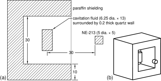
Figure 1: Monte Carlo geometry. All dimensions in cm. (a) Section view. (b) Perspective view.

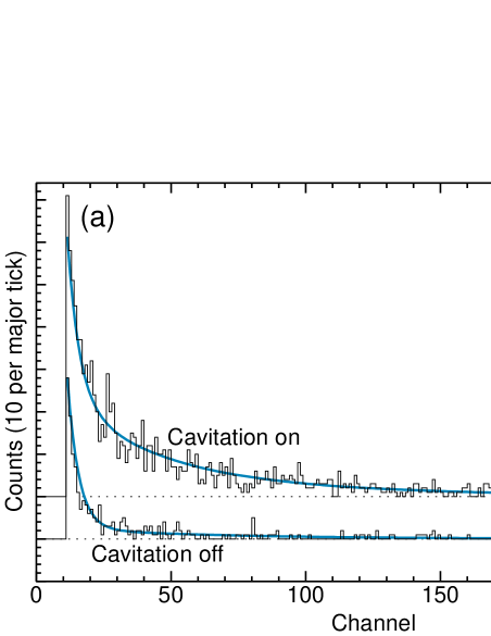
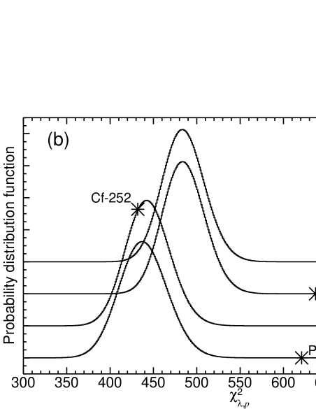
Figure 2: Fit statistics. (a) Fit using the simulated ${}^{252}\mbox{Cf}$ response function for $g_{k}$. The histograms are $n_{k}$ and $n^{\prime}_{k}$, and the smooth blue lines are theoretical curves $y_{k}$ and $y^{\prime}_{k}$. The minimized value of $\chi^{2}_{\lambda,p}$ is 432. For clarity, the two graphs are offset by ten counts. (b) Numerically sampled distributions of $\chi^{2}_{\lambda,p}$ for the four hypotheses. Observed values of $\chi^{2}_{\lambda,p}$ are shown.

References

- (1) R. P. Taleyarkhan et al., EPAPS Document No. E-PRLTAO-96-019605.
- Agostinelli et al. (2003) S. Agostinelli et al., Nucl. Instr. and Meth. A 506, 250 (2003).
- Verbinski et al. (1968) V. V. Verbinski, W. R. Burrus, T. A. Love, W. Zobel, N. W. Hill, and R. Textor, Nucl. Instr. and Meth. 65, 8 (1968).
- Lajtai et al. (1990) A. Lajtai, P. P. Dyachenko, V. N. Kononov, and E. A. Seregina, Nucl. Instr. and Meth. A 293, 555 (1990).
- Anderson and Neff (1972) M. E. Anderson and R. A. Neff, Nucl. Instr. and Meth. 99, 231 (1972).
- Baker and Cousins (1984) S. Baker and R. D. Cousins, Nucl. Instr. and Meth. 221, 437 (1984).
- Taleyarkhan et al. (2006) R. P. Taleyarkhan, C. D. West, R. T. Lahey, Jr., R. I. Nigmatulin, R. C. Block, and Y. Xu, Phys. Rev. Lett. 96, 034301 (2006).
- James and Roos (1975) F. James and M. Roos, Comput. Phys. Comm. 10, 343 (1975).