Direct sample estimates of multidimensional quadratic statistical functions: application to the anisotropic KPZ equation

Abstract

We suggest a class of direct sample estimates for the two-point quadratic statistical functions of multidimensional data, which includes: estimates of the sample autocovariance function (AcF), sample mean square increment (also, structure) function, and the estimate of the power spectrum. The central estimate for the class is the sample AcF, which is constructed as to represent the finite Fourier transform of the periodogram estimate of the spectrum and is positive semidefinite. The estimate explicitly account for the anisotropy of the fields in all spatial directions and is illustrated on two examples: the morphology of the Grab nebula and the surface roughness generated as a solution of the anisotropic Kardar-Parisi-Zhang equation. We also provide an expression of the covariance of the sample AcF in the case of data assumed to be drawn from a two-dimensional Gaussian field with a known mean.

I Introduction

Despite the increased availability of multidimensional data, it appears that not much attention has been devoted to the problem of adequate and accurate direct estimation of simple quantities such as two-point, quadratic statistical functions. The latter include autocovariance (AcF) and autocorrelation functions, and the mean square increment (also structure) function. Among the monographs we are aware of, a good exception is Priestley (1981), where an estimate of the two-dimensional AcF is discussed in some detail. Specifically, for a given $N_{1}\times N_{2}$ matrix of real data $f_{x_{1}x_{2}}$, $x_{1}=1,2,\dots N_{1}$, $x_{2}=1,2,\dots N_{2}$, the autocovariance function is estimated in volume 2, chapter 9 of Priestley (1981) by

$$A_{\ast}(\vec{u})=\displaystyle\frac{1}{N_{1}N_{2}}\sum_{x_{1}=1}^{N_{1}-u_{1}}\sum_{x_{2}=1}^{N_{2}-u_{2}}\hat{f}_{x_{1},x_{2}}\;\hat{f}_{x_{1}+u_{1},x_{2}+u_{2}},$$ (1)

where $\vec{u}=(u_{1},u_{2})$, $\hat{f}_{x_{1}x_{2}}=\left(f_{x_{1}x_{2}}-\bar{f}\right)$ with $\bar{f}$ denoting the sample mean, $\bar{f}=(1/N_{1}N_{2})\sum_{x_{1}=1}^{N_{1}}\sum_{x_{2}=1}^{N_{2}}f_{x_{1}x_{2}}$. The expression is valid for $0\leq u_{1}\leq N_{1}-1$ and $0\leq u_{2}\leq N_{2}-1$ and is extended to the third quadrant using the AcF property of being even function. Formally, the latter replaces $u_{1}$ and $u_{2}$ in (1) by their absolute values. Note that this leaves $A_{\ast}(\vec{u})$ undefined in the second and the fourth quadrants. We shall call this estimate “the standard” 2d sample autocovariance function (SAcF) estimate.

For a homogeneous (stationary) random 2d field, $f(\vec{x})$, the spectral representation theorem asserts that its AcF and spectral density function (or simply the spectrum) are related by the Fourier transform,

$${\cal S}(\vec{k})=\left(\frac{1}{2\pi}\right)^{2}\sum_{x_{1}=-\infty}^{+\infty}\sum_{x_{2}=-\infty}^{+\infty}{\cal A}(\vec{x})e^{i\vec{x}\cdot\vec{k}},$$ (2)

where $\vec{k}=(k_{1},k_{2})$. We use calligraphic letters to distinguish the “true” spectra and AcFs from their estimates. The inverse transform of (2) reads:

$${\cal A}(\vec{x})=\int_{-\pi}^{\pi}\int_{-\pi}^{\pi}{\cal S}(\vec{k})e^{-i\vec{x}\cdot\vec{k}}d^{2}k.$$ (3)

Equations (2) and (3) apply to a random field, which depends on discretely valued vector variable. It is desirable to have estimates that are also related by a (discrete and finite) Fourier transform. The simplest direct estimate of the spectrum is provided by the periodogram

$$I(\vec{k})=\frac{1}{(2\pi)^{2}N_{1}N_{2}}\sum_{x_{1},y_{1}=1}^{N_{1}-1}\sum_{x_{2},y_{2}=1}^{N_{2}-1}\hat{f}_{x_{1}x_{2}}\hat{f}_{y_{1}y_{2}}e^{-i\vec{k}\cdot(\vec{x}-\vec{y})}.$$ (4)

The periodogram, referred to as “raw” (unsmoothed) estimate, is a basis for variety of more sophisticated spectral estimates. Hence, in accordance with (3), we would like to have an AcF direct estimate, which for all $0\leq|u_{1}|\leq N_{1}-1$ and $0\leq|u_{2}|\leq N_{2}-1$ satisfies

$$A(\vec{u})=\int_{-\pi}^{\pi}\int_{-\pi}^{\pi}I(\vec{k})e^{-i\vec{k}\cdot\vec{u}}d^{2}k.$$ (5)

The standard estimate, $A_{\ast}$, satisfies (5), in the domains where it is defined. However, it is easy to see that if the validity of (1) is extended to the second and the fourth quadrants, Eq. (5) does not hold. The latter follows also from the developments presented in the next section.

Another property of the theoretical AcF that must be shared by an estimate is the property of positive semidefiniteness. Let $a_{x_{1},x_{2}}$ be an arbitrary non-zero $\left(N_{1}\times N_{2}\right)$ matrix of real numbers. Then the AcF of a 2d stationary field satisfies

$$\sum_{x_{1},y_{1}=1}^{N_{1}}\sum_{x_{2},y_{2}=1}^{N_{2}}a_{x_{1},x_{2}}a_{y_{1},y_{2}}{\cal A}\left(x_{1}-y_{1},x_{2}-y_{2}\right)\geq 0.$$ (6)

It easy to see that $A_{\ast}$ does not satisfy (6) in the second and the fourth quadrants. We stress that the inequality (6) does not bear theoretical importance only; it ensures the positiveness of spectral estimates based on an AcF estimate (indirect estimates) Percival and Walden (1995), see also Eq. (9) below.

In this paper we obtain a 2d AcF direct estimate, denoted hereinafter by $A(\vec{u})$, which satisfies (5) in all four quadrants, see the next section – Eq. (8). The estimate is identical to $A_{\ast}(\vec{u})$ in the first and the third quadrants but differs in the second and the fourth quadrants. The estimate $A(\vec{u})$ is positive semidefinite and leads to new estimates of both the mean square increment (structure) function and the power spectrum. We briefly discuss these estimates also in the second section and provide generalization of (8) for arbitrary dimension.

One of the most important advantages of the new estimate lays in the fact that it is capable to capture the anisotropy of the data in arbitrary spatial direction. The latter dictates the choice of the illustrations and applications we consider here; yet another application — a study of an YBCO thin film morphology using (8) — can be found in Atanasov et al. (2006). In the first of the two applications, we study the AcF of images representing the morphology of the Crab nebula. The random field for these images is the light intensity in a recorded pixel. The anisotropy in this case is determined either by the direction of the expansion of the supernova ejecta or by the interaction of synchrotron nebula with the ejecta Hester et al. (1996); Sankrit et al. (1998).

In the third section we compute the covariance of $A(\vec{u})$ for dimension $d=2$ and under the simplifying assumptions that the observations are drawn from a Gaussian random field and are already adjusted to have zero mean. Our second application involves the anisotropic Kardar-Parisi-Zhang (AKPZ) equation Villain (1991); Wolf (1991); Barabási and Stanley (1995), considered in section four in somewhat more detail. The equation pertains to growth of vicinal surfaces and the anisotropy arises from the different rates of growth along and across the average steps direction Villain (1991). We study how this anisotropy imprints on the shape of the AcF by numerically solving the AKPZ equation on a large lattice and then taking a smaller size images rotated on various angles with respect to the axis of anisotropy. A summary of our results and main conclusions are presented in the last section.

II Sample estimates of the multidimensional AcF

In order to obtain a direct estimate of the 2d sample AcF that corresponds to $I(\vec{k})$, we simply need to rearrange (4) to a 2d discrete Fourier transform. We begin by changing $y_{1}=x_{1}-u_{1}$ and reversing the order of $x_{1}$ and $u_{1}$ summation. This breaks up the sums with respect to $x_{1},y_{1}$ to two double sums: $\sum_{x_{1}=1}^{N_{1}}\sum_{y_{1}=1}^{N_{1}}=\sum_{x_{1}=1}^{N_{1}}\sum_{u_{1}=x_{1}\!-\!1}^{x_{1}-N_{1}}=\sum_{u_{1}=-(N_{1}\!-\!1)}^{0}\sum_{x_{1}=1}^{N_{1}+u_{1}}\;+\;\sum_{u_{1}=1}^{N_{1}-1}\sum_{x_{1}=1+u_{1}}^{N_{1}}$. Next, we shift the summation $x_{1}\mapsto x_{1}+u_{1}$ in the second term only obtaining the intermediate result:

$$I(\vec{k})=\frac{1}{(2\pi)^{2}N_{1}N_{2}}\sum_{x_{2},y_{2}=1}^{N_{2}} \Bigg{\{} \sum_{u_{1}=-(N_{1}\!-\!1)}^{0}\sum_{x_{1}=1}^{N_{1}-|u_{1}|}\hat{f}_{x_{1},x_{2}}\hat{f}_{x_{1}+|u_{1}|,y_{2}}\;e^{-i[k_{1}u_{1}+k_{2}(x_{2}-y_{2})]}$$

$$+ \sum_{u_{1}=1}^{N_{1}-1}\sum_{x_{1}=1}^{N_{1}-|u_{1}|}\hat{f}_{x_{1}+|u_{1}|,x_{2}}\hat{f}_{x_{1},y_{2}}\;e^{-i[k_{1}u_{1}+k_{2}(x_{2}-y_{2})]}\Bigg{\}}.$$

In analogous manner we deal with the $x_{2}$, and $y_{2}$ summations obtaining four terms, which then can be combined into two pairs arriving at the following 2d discrete Fourier representation of the periodogram

$$I(\vec{k})=\frac{1}{(2\pi)^{2}}\sum_{u_{1}=-N_{1}+1}^{N_{1}-1}\sum_{u_{2}=-N_{2}+1}^{N_{2}-1}A(\vec{u})\;e^{-i\vec{k}\cdot\vec{u}}.$$ (7)

In (7), we introduced the function

$$A(\vec{u})=\left\{\begin{array}[]{l}\displaystyle\frac{1}{N_{1}N_{2}}\sum_{x_{1}=1}^{N_{1}-|u_{1}|}\sum_{x_{2}=1}^{N_{2}-|u_{2}|}\hat{f}_{x_{1},x_{2}}\;\hat{f}_{x_{1}+|u_{1}|,x_{2}+|u_{2}|}\qquad\mbox{for $u_{1}\cdot u_{2}\geq 0$}\\ \displaystyle\frac{1}{N_{1}N_{2}}\sum_{x_{1}=1}^{N_{1}-|u_{1}|}\sum_{x_{2}=1}^{N_{2}-|u_{2}|}\hat{f}_{x_{1},x_{2}+|u_{2}|}\;\hat{f}_{x_{1}+|u_{1}|,x_{2}}\qquad\mbox{for $u_{1}\cdot u_{2}<0$},\end{array}\right.$$ (8)

which represents the new estimate of the sample AcF in dimension two. It differs from the standard estimate (1) in the second and fourth quadrants only. We stress that by the virtue of its construction, it is (8) but not the standard estimate that is related to the periodogram by (7).

A different way to obtain $A(\vec{u})$ is to substitute $I(\vec{k})$ directly in Eq. (5) and perform the integration with respect to $\vec{k}$. Then to use the obtained pair of Kronecker symbols to carry out two of the summations carefully accounting for the limits of summation. The latter depends on the position of $\vec{u}$, which produces (8).

The estimate $A(\vec{u})$ is positive semidefinite function. This follows from the way it was obtained but it is instructive to show that the positive semidefiniteness virtually forces the form of the SAcF, Eq. (8). To demonstrate this we use a 2d generalization of a proof of semidefiniteness due to McLeod and Jiménez, see Percival and Walden (1995), chapter 6. Let $\varepsilon_{x_{1},x_{2}}$ be a 2d white noise with zero mean and variance $1/N_{1}N_{2}$. Form a the field $g_{x_{1},x_{2}}=\sum_{k=1}^{N_{1}}\sum_{l=1}^{N_{2}}\hat{f}_{k,l}\varepsilon_{x_{1}-k,x_{2}-l}$; here the centered values of the sample, $\hat{f}_{k,l}$, are considered as coefficients of a moving average-like 2d field. Since $g_{x_{1},x_{2}}$ is stationary, its theoretical AcF must be positive semidefinite. A straightforward calculation shows that this function is given by (8). One last remark regarding (8): it easy to see that the estimate $A(\vec{u})$ can be computed numerically using the FFT-based algorithm and the codes given in Press et al. (1992), chapters 12 and 13; however, by first extending the data twice in both dimensions and assuming that $f_{x_{1},x_{2}}\equiv 0$ if either $N_{1}\leq x_{1}\leq 2N_{1}$, or $N_{2}\leq x_{2}\leq 2N_{2}$ (double length zero padding).

Estimate (8) can be used as a basis for estimates of both sample power spectrum and sample mean square increment function. One can obtain an estimate of the spectrum from (8) by employing it in a 2d generalization of Grenander and Rosenblatt formula Grenander and Rosenblatt (1957),

$$S(\vec{k})=\frac{1}{(2\pi)^{2}}\sum_{u_{1}=-N_{1}+1}^{N_{1}-1}\sum_{u_{2}=-N_{2}+1}^{N_{2}-1}w(\vec{u})A(\vec{u})e^{-i\vec{k}\cdot\vec{u}},$$ (9)

where the function $w(\vec{u})$ is termed “lag window”. The general properties and specific examples of $w(\vec{u})$ can be found in Priestley (1981); we note here that obviously it must be an even function $w(-\vec{u})=w(\vec{u})$. The statistics of this estimate will be presented elsewhere, note however that as in the 1d case, (5) provides a smoothed compared to the “raw” periodogram estimate.

The mean square increment (structure) function of $f(\vec{x})$, ${\cal B}(\vec{u})$, is defined Berry (1979); Panchev (1971) by ${\cal B}(\vec{u})=E\left[\left(f(\vec{x}+\vec{u})-f(\vec{x})\right)^{2}\right]$, where $E$ denotes the ensemble averaging, and is related to the AcF by ${\cal B}(\vec{u})=2\left({\cal A}(0)-{\cal A}(\vec{u})\right)$, e.g. Yordanov and Atanasov (2002); for an estimate that corresponds to the standard estimate of ${\cal A}(\vec{u})$ see Russ (1994); Thomas et al. (1999). An estimate corresponding to (8) should be modified in the second and the fourth quadrants as:

$$B(\vec{u})=\frac{1}{N_{1}N_{2}}\sum_{x_{1}=1}^{N_{1}-|u_{1}|}\sum_{x_{2}=1}^{N_{2}-|u_{2}|}\left(f_{x_{1},x_{2}+|u_{2}|}-f_{x_{1}+|u_{1}|,x_{2}}\right)^{2},\qquad\mbox{for $u_{1}\cdot u_{2}<0$}.$$ (10)

In addition of being a positive function, we remark that $B(\vec{u})$ does not involve the sample mean of $f(\vec{x})$ and thus is free from a source of bias brought up by $\overline{f}$ Box and Jenkins (1976); Percival and Walden (1995). Modifications analogous to (10) are apparently due for the estimates of the generalized structure functions used to infer multifractal scaling, see Refs. Barabási and Vicsek (1991); Krug (1994).

Estimate (8) can readily be generalized to arbitrary dimension $d$. To shorten the notations, consider a multi-index with $d$ components $p=(p_{1},p_{1},\dotsc p_{d})$ each taking a value of either $0$ or $1$. Let $p_{k}=0$ indicates $x_{k}$, whereas $p_{k}=1$ indicates $x_{k}+|u_{k}|$, $k=1,2,\dotsc d$, and let $\overline{p}$ designate the multi-index whose components are all different from the components of $p$; e.g. if $p=(011)$, then $\overline{p}=(100)$. Then the $d$-dimensional SAcF estimate can be expressed as

$$A_{p}(\vec{u})=\frac{1}{N_{1}N_{2}\dotsc N_{d}}\sum_{x_{1}=1}^{N_{1}-|u_{1}|}\dotsb\sum_{x_{d}=1}^{N_{d}-|u_{d}|}\hat{f}_{p}\hat{f}_{\overline{p}},$$ (11)

where $p=(0,0,\dotsc,0)$ pertains to the first and the $2^{d-1}+1$-th hyperquadrants, $p=(0,0,\dotsc,1)$ to the second and $2^{d-1}+2$-th hyperquadrants, and so on. In general, the SAcF in hyperquadrants $k$ and $2^{d-1}+k$ is expressed by (11) with a multi-index p, which is the binary representation of number $k-1$.

To illustrate the difference between the standard and the estimate (8), we provide plots of both estimates for pair of images representing regions of the Crab nebula. The images were selected from a color image taken from the Hubble Space Telescope (HST) www . The color image was created as a weighted sum of three narrowband filters centered at 5012 Å, 6306 Å and 6732 Å and comprises 24 individual Wide Field and Planetary Camera 2 exposures Hester et al. (1996). We converted the color image into gray scale (in the range of 0-256) image, i.e. $f_{x,y}$ in this case is proportional to the light intensity per pixel and represents the morphology of the nebula; we added a circle indicating the position of the Crab pulsar. The first of the selected images, shown in Fig. 1(b) top panel, is located close to outer rim of the nebula dominated by the expanding ejecta Hester et al. (1996); Sankrit et al. (1998). The coordinates of its right bottom corner are, RA: $\alpha_{2000}=$5:34:40.5 and Dec: $\delta_{2000}=$21:59:39.1. The image extends (46.2$\times$49.7) arcseconds corresponding to $(N_{1}=453)\times(N_{2}=487)$ pixels. By just inspecting the image the anisotropy is not easily recognizable, however, due to the outward expansion of the supernova remnant an anisotropy roughly across the radial direction (direction to the pulsar) should present in the morphology.

The second image has coordinates: $\alpha_{2000}=$5:34:29.0, $\delta_{2000}=$ 21:59:10.0 and extends 51.8$\times$51.8 arcseconds, ($504\times 504$) pixels — Fig. 1(b), bottom panel. It is from a region where the synchrotron nebula (upper left sector of the image) interacts with the denser ejecta creating “filaments”. The latter are attributed to a magnetic Rayleigh-Taylor (R-T) instabilities Hester et al. (1996). The major axis of anisotropy in this region should, in general, be expected along rather then across the direction to the pulsar.

           

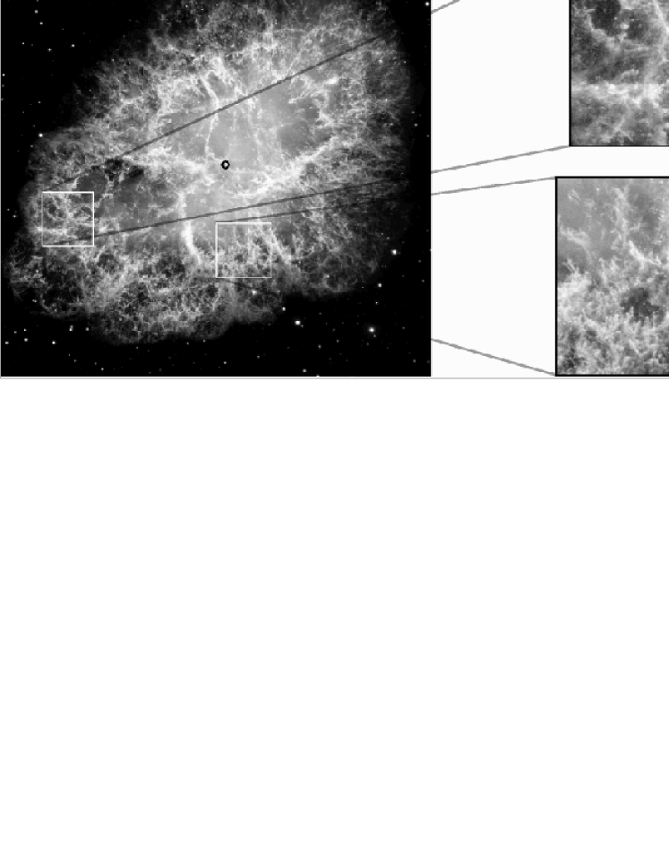
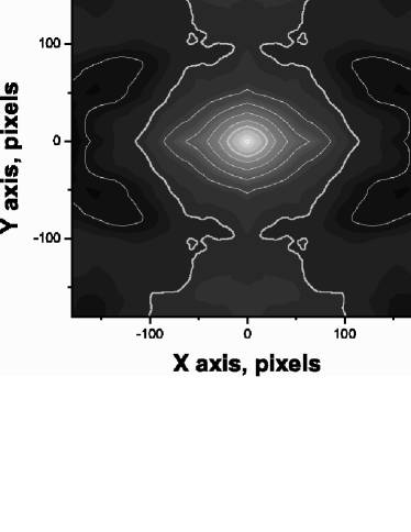
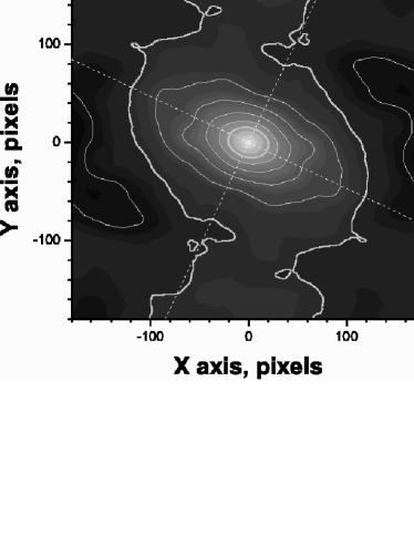
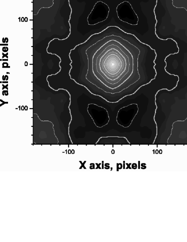
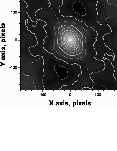
(a)                                                                      (b)

(c)                                                              (d)

(e)                                                              (f)

Figure 1: Standard AcF estimate and estimate (8) for two regions of the Crab nebula. Panel (a) shows the location of the regions; the circle indicates the position of the pulsar. Panel (b) shows the two regions zoomed by an identical factor. Panels (c) and (d) show the standard AcF estimate and the estimate (8), respectively for the upper image in (b). Panels (e) and (f) – the same the bottom image in (b). The morphology principle axes of anisotropy are drawn in plates (d) and (f).

An overall linear (planar) trend, $g=s_{\alpha}\alpha+s_{\delta}\delta$ with origins of coordinate systems at the left-upper corners of the images, is removed before both SAcF estimates were computed. Carrying out this procedure is important since the trend by itself produces anisotropy in the SAcF. In the case of images presented in Fig. 1(b) the linear trend is rather small; the estimated slopes (in units grayscale/pixel) are $s_{\text{DEC}}=-0.027$, $s_{\text{RA}}=0.0071$, and $s_{\text{DEC}}=0.101$, $s_{\text{RA}}=0.031$, for first and second images, respectively. The standard and the estimate (8) for the first image are presented as gray scale plots with superimposed level contours in Fig. 1(c) and Fig. 1(d), respectively. For the sake of completeness of the plot the standard AcF is extended to the second and the fourth quadrants, hence the specific “rose” appearance of the AcF. The anisotropy of the supernova remnant structures in this part of the nebula is clearly recognized from the plot of $A(\vec{u})$ with the major axis of anisotropy having an angle of about $\vartheta\approx-25^{\circ}$ with respect to the horizontal axis. This angle should be interpreted as the average front of the local expansion, refer to Fig. 1(a). Another quantity that characterizes the anisotropy is the aspect ratio, $\gamma$, the ratio between the characteristic sizes of the nebula structures along the minor and majors axes of anisotropy. The latter sizes are defined by the correlation lengths of SAcF in the respective directions. We evaluate these lengths crudely by assuming, somewhat arbitrary, that the 1d principal profiles of AcF are represented by random processes with finite domain (band-limited) spectra. Using the expressions for the correlation length obtained for this class of random processes in Yordanov and Nickolaev (1994, 1997), we infer $\gamma\approx 0.57$.

For the second region, the major axis of the anisotropy is at angle of $\vartheta\approx-59.5^{\circ}$ with respect to the horizontal axis, which as should be expected is roughly in direction to the pulsar, refer to Fig. 1(a) and Fig. 1(f). The aspect ratio in this case is $\gamma\approx 0.875$.

III Covariances of the 2d sample autocovariance function

In this section we obtain expression for covariances of 2d SAcF — the estimate (8), evaluated at two points $\vec{u}=(u_{1},u_{2})$ and $\vec{v}=(v_{1},v_{2})$:

$$\text{cov}\big{[}A(\vec{u}),A(\vec{v})\big{]}=E\big{[}A(\vec{u})A(\vec{v})\big{]}-E\big{[}A(\vec{u})\big{]}E\big{[}A(\vec{v})\big{]}.$$ (12)

The covariance has both theoretical as well as practical importance for determining the confidence intervals in the AcF estimate. The expression will be derived under the simplifying assumptions that $f_{x_{1},x_{2}}$ is a Gaussian random field with zero mean (or that the mean is known and subtracted). It is immediately seen that irrespective to which quadrant $\vec{u}$ belongs,

$$E\big{[}A(\vec{u})\big{]}=\left(1-\frac{|u_{1}|}{N_{1}}\right)\left(1-\frac{|u_{2}|}{N_{2}}\right){\cal A}(\vec{u}),$$ (13)

where as before ${\cal A}(\vec{u})$ denotes the true autocovariance function of $f(\vec{x})$. Eq. (13) is identical to the ensemble average of the standard estimate and shows that (8) is a biased estimate. The bias, however, is small for large samples especially for small $|\vec{u}|$. We turn now to the first term in (12). Reckoning with $A(-\vec{u})=A(\vec{u})$ and the symmetry under the exchange $\vec{u}\leftrightarrow\vec{v}$, we need to consider three different cases only: (i) $\vec{u}\in$ I quadrant, $\vec{v}\in$ I quadrant; (ii) $\vec{u}\in$ II quadrant, $\vec{v}\in$ II quadrant; and (iii) $\vec{u}\in$ I quadrant, $\vec{v}\in$ II quadrant. The calculations in all three cases are closely similar; below we illustrate them for the case (ii) only. Inserting the pertinent for this case AcF expressions from (8) and using that for a Gaussian field the four-point function can be expressed as combinations of products of two two-point AcFs we have

$$E\big{[}A(\vec{u})A(\vec{v})\big{]} = \frac{1}{N_{1}^{2}N_{2}^{2}}\sum_{x_{1}=1}^{N_{1}-|u_{1}|}\sum_{x_{2}=1}^{N_{2}-|u_{2}|}\sum_{y_{1}=1}^{N_{1}-|v_{1}|}\sum_{y_{2}=1}^{N_{2}-|v_{2}|}\Big{[}{\cal A}(|u_{1}|,-|u_{2}|){\cal A}(|v_{1}|,-|v_{2}|)$$

$$+{\cal A}(y_{1}\!-\!x_{1},y_{2}\!-\!x_{2}\!+\!|v_{2}|\!-\!|u_{2}|){\cal A}(y_{1}\!-\!x_{1}\!+\!|v_{1}|\!-\!|u_{1}|,y_{2}\!-\!x_{2})$$

$$+{\cal A}(y_{1}\!-\!x_{1}\!+\!|v_{1}|,y_{2}\!-\!x_{2}\!-\!|u_{2}|){\cal A}(y_{1}\!-\!x_{1}\!-\!|u_{1}|,y_{2}\!-\!x_{2}\!+\!|v_{2}|)\Big{]}.$$

The first of these terms does not depends of the summation indexes and cancels out with the second term in (12) exactly, refer to (13). In the remaining two terms we perform the indicated change $\vec{p}=\vec{y}-\vec{x}$ and again reverse the order of the summation. This allows to carry out the summations with respect to both $x_{1}$ and $x_{2}$ explicitly, noting in the process that we need to distinguish the case $|u_{1}|>|v_{1}|$ from the case $|v_{1}|>|u_{1}|$. The result is a product of two trapezium shaped functions, which involve two parameters, $c$ and $d$,

$$W(c,d;p):=\left\{\begin{array}[]{rrcl}0,&\quad\!&\!p\!&\!\leq-(1-c)\\ 1-c+p,&\quad-(1-c)\leq\!&\!p\!&\!\leq-d\\ 1-c-d,&\quad-d\leq\!&\!p\!&\!\leq d\\ 1-c-p,&\quad d\leq\!&\!p\!&\!\leq 1-c\\ 0,&\quad 1-c\leq\!&\!p\!&\!,\end{array}\right.$$ (15)

see also Fig. 2. The parameters $c$ and $d$ are subject to the conditions $0\leq d\leq 1-c\leq 1$.

Figure 2: Graph of the window function $W(c,d;p)$, Eq. (15), used in the expression of the sample AcF covariances.

Next, introducing $\vec{a}:=(\vec{u}+\vec{v})/2$; $\;\vec{b}:=(\vec{u}-\vec{v})/2$ and shifting the summation indexes $p_{1}$ and $p_{2}$ simultaneously according to $\vec{p}=(q_{1}-u_{1}-N_{1},q_{2}+u_{2}-N_{2})$, we arrive at the following expression for the covariance valid when both $\vec{u}$ and $\vec{v}$ are in the second quadrant:

$$\mbox{cov}\Big{[}A(\vec{u}),A(\vec{v})\Big{]} = \frac{1}{N_{1}N_{2}}\sum_{q_{1}=1}^{2N_{1}+2a_{1}-1}\;\sum_{q_{2}=1}^{2N_{2}-2a_{2}-1}W\left(-\frac{a_{1}}{N_{1}},\frac{|b_{1}|}{N_{1}};\frac{r_{1}}{N_{1}}\right)W\left(\frac{a_{2}}{N_{2}},\frac{|b_{2}|}{N_{2}};\frac{r_{2}}{N_{2}}\right)$$ (16)

$$\times\Big{[}{\cal A}(\vec{r}+\vec{a})\;{\cal A}(\vec{r}-\vec{a})+{\cal A}(\vec{r}+\vec{b})\;{\cal A}(\vec{r}-\vec{b})\Big{]},$$

where $\vec{r}=(q_{1}-a_{1}-N_{1},q_{2}+a_{2}-N_{2})$ has been introduced.

Similar expressions are obtained in cases (i) and (iii) above. Finally, if we define $\widetilde{a}_{1,2}:=(|u_{1,2}|+|v_{1,2}|)/2$ and $\widetilde{b}_{1,2}:=(|u_{1,2}|-|v_{1,2}|)/2$, all three cases can be combined into the following compact form:

$$\mbox{cov}\Big{[}A(\vec{u}),A(\vec{v})\Big{]} = \frac{1}{N_{1}N_{2}}\sum_{q_{1}=1}^{2N_{1}-2\widetilde{a}_{1}-1}\;\sum_{q_{2}=1}^{2N_{2}-2\widetilde{a}_{2}-1}W\left(\frac{\widetilde{a}_{1}}{N_{1}},\frac{|\widetilde{b}_{1}|}{N_{1}};\frac{r_{1}}{N_{1}}\right)W\left(\frac{\widetilde{a}_{2}}{N_{2}},\frac{|\widetilde{b}_{2}|}{N_{2}};\frac{r_{2}}{N_{2}}\right)$$ (17)

$$\times\Big{[}{\cal A}(\vec{r}+\vec{a})\;{\cal A}(\vec{r}-\vec{a})+{\cal A}(\vec{r}+\vec{b})\;{\cal A}(\vec{r}-\vec{b})\Big{]},$$

with the general definition $\vec{r}=(q_{1}+\widetilde{a}_{1}-N_{1},q_{2}+\widetilde{a}_{2}-N_{2})$. This expression is valid for arbitrary positions of vectors $\vec{u}$ and $\vec{v}$.

The important for the practice variances of the SAcF, can be obtained from the expressions of the covariance. Setting $\vec{v}=\vec{u}$ in (17) we have

$$\mbox{var}\left[A(\vec{u})\right] = \frac{1}{N_{1}N_{2}}\sum_{p_{1}=-N_{1}\!+\!|u_{1}|\!+\!1}^{N_{1}\!-\!|u_{1}|\!-\!1}\;\sum_{p_{2}=-N_{2}\!+\!|u_{2}|\!+\!1}^{N_{2}\!-\!|u_{2}|\!-\!1}\left(1-\frac{|u_{1}|+|p_{1}|}{N_{1}}\right)\left(1-\frac{|u_{2}|+|p_{2}|}{N_{2}}\right)$$ (18)

$$\times \Big{[}\mathcal{A}^{2}\big{(}p_{1},p_{2}\big{)}\;+\;\mathcal{A}\big{(}p_{1}\!+\!|u_{1}|,p_{2}\!+\!|u_{2}|\big{)}\;\mathcal{A}\big{(}p_{1}\!-\!|u_{1}|,p_{2}\!-\!|u_{2}|\big{)}\Big{]}.$$

Note that we went back from summation with respect to $q_{1}$ and $q_{2}$ to summation with respect to $p_{1}$ and $p_{2}$, which results in symmetric about zero limits of summation.

IV Application to the anisotropic KPZ equation

The anisotropic Kardar-Parisi-Zhang (AKPZ) equation has been introduced in an attempt to model the growth on a vicinal substrates Villain (1991). Adatoms that migrate towards the steps and attach to them, have lower probability to desorb compared to those migrating parallel to the steps. This effectively induces different rates of growth along and across the steps and violates the rotational symmetry of the KPZ growth process Kardar et al. (1986). Let $h=h(\vec{x},t)$ be the height of the growing surface at point $\vec{x}=(x,y)$ and time $t$. If one chooses the $x$-coordinate along the direction of the steps, the AKPZ equation takes the form:

$$\partial_{t}h=\nu_{x}\partial_{x}^{2}h+\nu_{y}\partial_{y}^{2}h+\frac{\lambda_{x}}{2}\left(\partial_{x}h\right)^{2}+\frac{\lambda_{y}}{2}\left(\partial_{y}h\right)^{2}+\eta,$$ (19)

see also Barabási and Stanley (1995). In this equation: $\nu_{x}$ and $\nu_{y}$ are coefficients of the curvature terms associated with desorption, $\lambda_{x}$ and $\lambda_{y}$ are coefficients related to growth rates normal the surface, and $\eta=\eta(x,y,t)$ is a Gaussian white noise, $E[\eta(x,y,t)\eta(x^{\prime},y^{\prime},t^{\prime})]=2D\delta(x-x^{\prime})\delta(y-y^{\prime})\delta(t-t^{\prime})$. The equation has been studied by D. E. Wolf using one-loop, renormalization-group (RG) approximation Wolf (1991). Some of the obtained results have later been confirmed by numerical simulations Halpin-Healy and Assdah (1992). To recap what will be needed here, let $r_{\nu}=\nu_{y}/\nu_{x}$ and $r_{\lambda}=\lambda_{y}/\lambda_{x}$ and let both $\lambda_{x}$ and $\lambda_{y}$ be positive. In this case the AKPZ surface grows with an exponent identical to the surface generated by the isotropic KPZ equation, referred to as algebraic roughness. As the morphology evolves, the nonlinear parameters $\lambda_{x}$ and $\lambda_{y}$, as in the case of isotropic KPZ are not renormalized, whereas $\nu_{x}$ and $\nu_{y}$ take effective values such that $r_{\nu}=r_{\lambda}$ (a fixed point to the dynamical renormalization flow equations) Wolf (1991). This means that in this case the anisotropy of the surface is of the simplest kind – elliptical anisotropy – and therefore might be taken as a benchmark for testing statistical methods characterizing anisotropy.

The numerical simulations were carried out using the Amar and Family numerical scheme Amar and Family (1990); Chakrabarti and Toral (1989); Keye et al. (1991), which broadly speaking includes rescaling of the equation and employing the standard discretization for the derivatives. Two comments are in order. First, in contrast to Halpin-Healy and Assdah (1992), we choose rescaling that leaves the equation manifestly anisotropic: $x\mapsto\sqrt{\nu_{x}}x$, $y\mapsto\sqrt{\nu_{x}}y$, $h\mapsto(2\nu_{x}/\lambda_{x})h$, and $\eta\mapsto\sqrt{2D/\nu_{x}}\eta$. Second, the discrete analog does not adequately represent the continuous AKPZ equation Lam and Shin (1998a), however, since more accurate difference scheme are not known for dimensions higher than one Lam and Shin (1998b); Buceta (2005), we employ here the standard discretization. What is more important within the scope of this study, the discrete equation inherits the elliptical anisotropy of the original AKPZ equation.

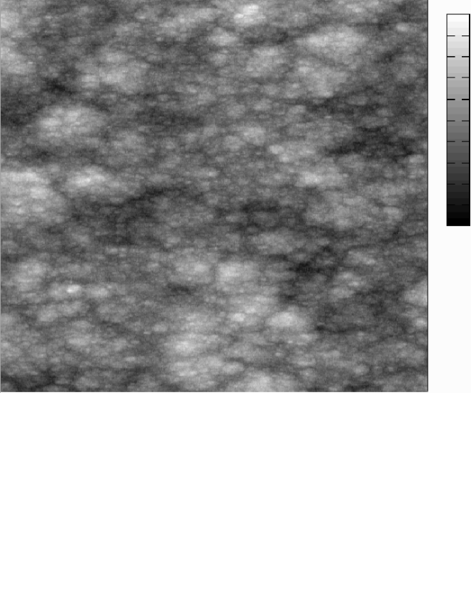
Figure 3: Gray scale image of a morphology obtained by numerically solving the anisotropic KPZ equation. The image represents the central (512$\times$512) part from the entire (1024$\times$1024) simulated surface. The conditions at which the simulation is carried out are discussed in the text.

The elliptical anisotropy can be discerned even by visually inspecting of the simulated morphology, see Fig. 3. The picture represents AKPZ surface generated with parameters $\nu_{x}=1$, $\nu_{y}=0.3$, $\lambda_{x}=10$, $\lambda_{y}=3$, and $D=0.2$; (to skip the “transient” time for the system to come to the RG fixed point, we have chosen $r_{\nu}=r_{\lambda}=0.3$ at the outset). The simulation is carried out on a square lattice with side of $L=1024$ and for $T=2\times 10^{5}$ time steps of $\Delta t=0.001$. The surface height range is given in units of lattice spacing set to unity.

In a typical experimental circumstances, the axes of anisotropy are rarely known and need to be inferred and quantified from a image of the morphology Thomas et al. (1999). To reckon with this we “record” smaller, (512$\times$512), images, which are rotated at angles $\psi_{0}=0^{\circ}$, $10^{\circ}$, $30^{\circ}$, and $60^{\circ}$ with respect to the $x$-axis of the simulated surface. The picture in Fig. 3 represents the image for $\psi_{0}=0^{\circ}$. The images for $\psi_{0}\neq 0^{\circ}$ are obtained using a simple, based on the four nearest neighbor points interpolation. Then for every image we compute the AcF estimate (8), an example of which for $\psi_{0}=30^{\circ}$ is shown in Fig. 4. Taking a more systematic approach, rather than the correlation length, we consider sections of AcF defined by $aA(0)\leq A(\vec{u})\leq(a+\Delta{a})A(0)$ for several levels $0<a<1$ and a fixed width of $\Delta a=0.04$. We project the values of $A(\vec{u})$ within each section on the $(u_{1},u_{2})$ plane and fit these points by an ellipse. The direction of the axis of asymmetry and the aspect ratio is evaluated from the parameters of these ellipses. In the actual fits we have used four levels of $a$: 0.2, 0.4, 0.6, and 0.8.

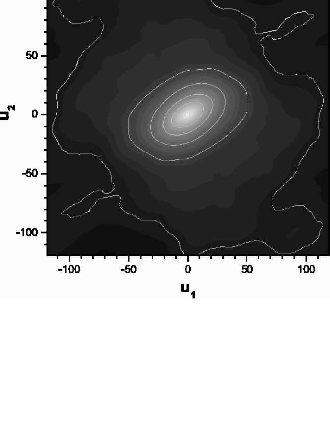
Figure 4: Sample AcF for an image of the AKPZ simulated morphology illustrated in Fig. 3, however rotated on angle $30^{\circ}$.

The obtained results show a discrepancy typically within $\pm 2^{\circ}$ from the expected direction of the anisotropy. In few cases only, all associated with the lowest level of $a$, the discrepancy is up to $\pm 4^{\circ}$. More interesting are the inferred values of the aspect ratio. These are plotted in Fig. 5 for all four angles of rotation and AcF levels $a$ and for two simulated surfaces, studied independently. The parameters of the first simulation are the same as those used to produce Fig. 3. The lattice size, the time step, and total integration time for the second simulation are also the same, however, with: $\nu_{x}=1$, $\nu_{y}=0.15$, $\lambda_{x}=10$, $\lambda_{x}=1.4$, and $D=0.2$ ($r_{\nu}=r_{\lambda}=0.15$). The values of $\gamma$ for the first simulation are grouped around $0.548$, upper part of the figure, whereas for the second — around $0.387$ bottom part of the figure. Both these values correspond to the respective $\sqrt{r_{\nu}}$ values used in the simulations. To understand this, we rescale (19) in a manner different from the one used prior to numerical integration; namely, $x=\sqrt{\nu_{x}}\widetilde{x}$, $y=\sqrt{\nu_{y}}\widetilde{y}$, $h=\left(\sqrt{2D}/\nu_{x}^{1/4}\nu_{y}^{1/4}\right)\widetilde{h}$, and $\eta=(\sqrt{2D}/\nu_{x}^{1/4}\nu_{y}^{1/4})\widetilde{\eta}$, arriving at

$$\partial_{t}\widetilde{h}=\partial_{\widetilde{x}}^{2}\widetilde{h}+\partial_{\widetilde{y}}^{2}\widetilde{h}+\frac{\varepsilon_{x}}{2}\left(\partial_{\widetilde{x}}\widetilde{h}\right)^{2}+\frac{\varepsilon_{y}}{2}\left(\partial_{\widetilde{y}}\widetilde{h}\right)^{2}+\widetilde{\eta}.$$ (20)

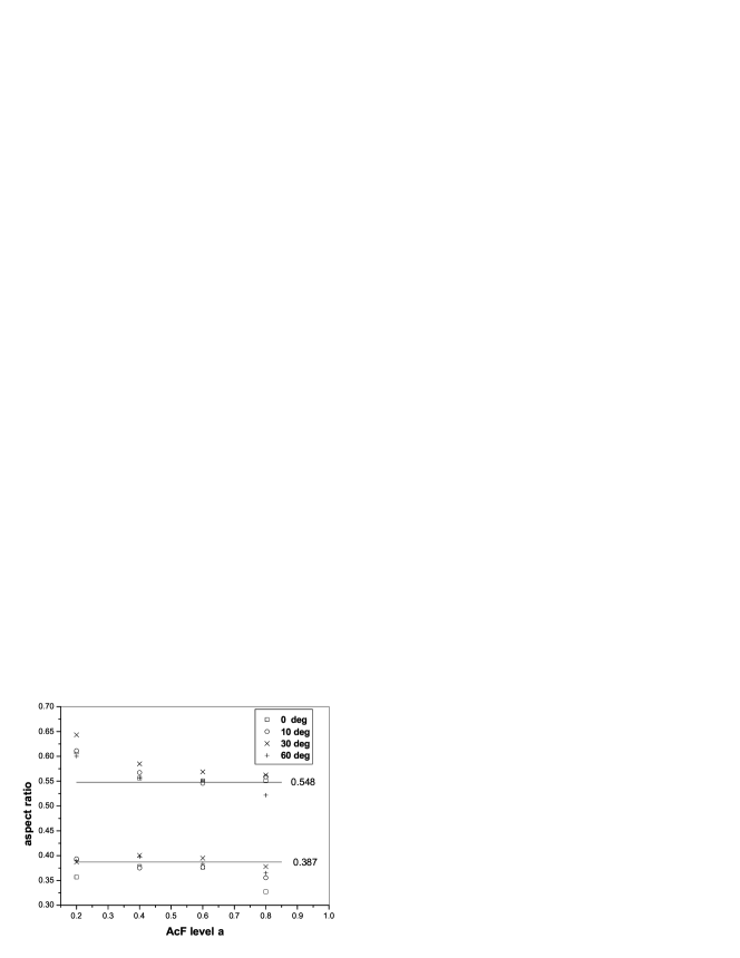
Figure 5: Retrieved aspect ratio $\gamma$ from four AcF sections marked by levels $a$ and for four angles of rotation of the recorded image, see the legends. Upper and bottom data represent results from two simulated surfaces, see the text. The horizontal lines indicate the expected values of the aspect ratio, $\gamma=\sqrt{\nu_{y}/\nu_{x}}$.

In the above equation, $\varepsilon_{x}=\lambda_{x}\sqrt{2D}/\nu_{x}^{3/2}r_{\nu}^{1/4}$ and $\varepsilon_{y}=\left(r_{\lambda}/r_{\nu}\right)\varepsilon_{x}$ and hence at the fixed point of the RG, Eq. (20) is equivalent to the isotopic KPZ equation. Therefore, the anisotropic surface in this case is obtained by just rescaling the isotropic surface in $x$ and $y$ directions by $l_{x}=\sqrt{\nu_{x}}$ and $l_{y}=\sqrt{\nu_{y}}$, respectively. The latter leads to aspect ratio of $\gamma=\sqrt{r_{\nu}}$, which as demonstrated in Fig. 5 is imprinted in the sample AcF, Eq. (8). A somewhat larger discrepancy from $\sqrt{r_{\nu}}$ observed at the lowest level fits can be attributed to a greater relative variability of the SAcF. The latter can be estimated crudely from the variance (18) by substituting the SAcF for the unknown true AcF. For the two simulations used in Fig. 5, we obtain an increase from 12% at $\vec{u}=0$, up to about 23% for points $\vec{u}$ at which $A(\vec{u})=0.2A(0)$. As a final remark, the one-loop RG approximation of the AKPZ equation indicates that if $\lambda_{y}\neq 0$ the surfaces in this class are characterized by two characteristic lengths, $l_{x}$ and $l_{y}$, even when the morphology has not yet evolved to the RG fixed point. In addition, the characteristic length scale linearly, $l_{y}\sim l_{x}$, Ref. Wolf (1991). This suggests that the approach undertaken in this section may be suitable for characterization of more generic AKPZ morphologies. Further numerical simulations, however, are needed to confirm this assertion.

V Conclusions

In this paper we have suggested an estimate for the autocovariance function (AcF) of a homogenous random field in arbitrary dimension $d$. The estimate, Eq. (11), is constructed as to represent the discrete and finite Fourier transform of the periodogram estimate of the field’s power spectrum; it is identical to the standard AcF estimate in the first and the $2^{d-1}+1$-th quadrants but differs in all other quadrants. As it should be, the estimate is positive semidefinite. On the basis of (11), we have suggested new estimates for the field’s structure function and power spectrum. We have also derived expressions for the covariance, consequently for the variance of the AcF estimate in two dimensions under the simplifying assumption that the field is Gaussian and with a known mean.

Perhaps the most important advantage of the new sample AcF over the standard estimate lays in the fact that it captures the anisotropy of the field in all spatial directions. The latter is demonstrated on two examples. The first involves the morphology of the Grab nebula observed by the Hubble space telescope. For sake of comparison we presented plots of the standard AcF as well. The second example involves surfaces simulated by numerically solving the anisotropic Kardar-Parisi-Zhang (AKPZ) equation and is considered in more detail. In particular, we have focused on the case $\nu_{y}/\nu_{x}=\lambda_{y}/\lambda_{x}$, i.e. when the system is at a fixed point of the dynamic renormalization group approximation for the AKPZ equation. In this case the characteristic lengths of the morphology are two and are determined by $l_{x}=\sqrt{\nu_{x}}$ and $l_{y}=\sqrt{\nu_{y}}$. Hence, the surface can be viewed as a simple benchmark for testing statistical methods that account for anisotropy. We have shown that one can retrieve both the direction and the aspect ratio of the anisotropy reasonably well from the estimate (11) in two dimensions. This has been done on several sections of the AcF and on two independent realizations.