Detecting the traders’ strategies in Minority-Majority games and real stock-prices.

Abstract

Price dynamics is analyzed in terms of a model which includes the possibility of effective forces due to trend followers or trend adverse strategies. The method is tested on the data of a minority-majority model and indeed it is capable of reconstructing the prevailing traders’ strategies in a given time interval. Then we also analyze real (NYSE) stock-prices dynamics and it is possible to derive an indication for the the “sentiment” of the market for time intervals of at least one day.

I Introduction

The simplest representation of price dynamics is usually considered as a simple Random Walk (RW). It is easy to realize, however, that many important deviations ara also present. The most studied are the problem of the “fat tails” (in the distribution of price returns), the volatility clustering and various other elements related to the non stationarity of the process mantegna-stanley ; bouchaud-potters . The arbitrage condition implies that no simple correlations can be present. A large effort is therefore devoted to the identification of complex correlations of various types. These correlations arise from the collective behavior of traders, which lastly, define the price.

In this perspective a simple classification of trading strategies can be made in terms of trend followers or trend adverse. Usually these different strategies are taken as input in models which represent the behavior of traders.

Here we would like to consider the complementary point of view. Namely, given a time series, is it possible to identify, from the data, the strategies of the traders? In order to address this question we use a new approach which is based on a RW plus a force which depends on the distance of the price from some suitable moving average vale1 ; taka1 . This idea is that, with such an analysis, one can identify the “sentiment” of the market in a given time interval.

In this paper, we first perform some statistical tests of the method to clear its signal to noise ratio. Then we apply the method to time series generated by a minority-majority model ameno . This is an important test because, in this case, one knows the prevailing strategy of the traders. The results are rather encouraging because the method can indeed identify these strategies. Finally we apply the method to real stock prices data of the NYSE and the preliminary results show that it is possible to derive statistically significant information on the prevailing trading strategy for a single day or larger time periods.

II The Effective Potential Model

In recent papers taka1 ; vale1 has been introduced the idea the the stock-price dynamics can be influenced by a moving average of the price itself in the previous time steps. Hence, at every time step $t$, one can introduce a moving average of the previous $M$ time steps:

$${P_{M}(t)}=\frac{1}{M}\sum_{\tau=0}^{M-1}{P(t-\tau)}$$ (1)

In Fig.  1 is plotted the time evolution of a RW with Gaussian random noise together with the moving average of the price.

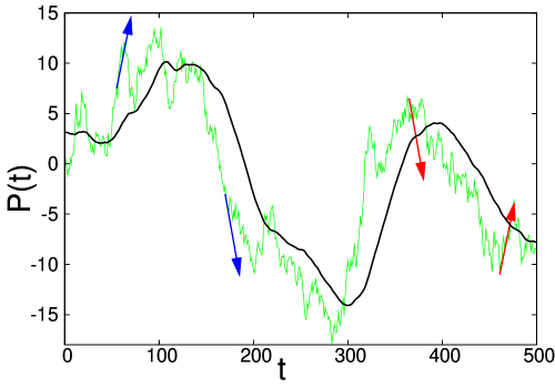
Figure 1: Example of a model of price dynamics (in this case a simple RW) together with its moving average defined as the average over the previous $50$ points. The idea is that the distance of the price from its moving average can lead to repulsive (blue arrows) or attractive (red arrows) effective forces.

One can investigate if there could be a relation between the next price increment $P(t+1)-P(t)$ and the difference $P(t)-P_{M}(t)$.

The simplest assumption is to adopt a linear dependence:

$$P(t+1)-P(t)\propto P(t)-P_{M}(t)$$ (2)

In this case, the price dynamics can be described in terms of a RW with the existence of a linear force. This force can be either repulsive or attractive depending on the sign of the constant of proportionality between $P(t+1)-P(t)$ and $P(t)-P_{M}(t)$.

Therefore, the dynamical equations of the price is a RW with the presence of a force that is the gradient of a quadratic potential $\Phi$ taka1 .

$$P(t+1)=P(t)-b(t)\frac{d}{dP(t)}\Phi\Big{(}P(t)-P_{M}(t)\Big{)}+\omega(t)$$ (3)

where $\omega(t)$ corresponds to a random noise with unitary variance and zero mean. $P_{M}(t)$ is the moving average described in Eq. 1.

The potential $\Phi$ together with the pre-factor $b(t)$ describe the interaction between the price and the moving average. In simple assumption of a linear force taka1 , $\Phi$ results to be quadratic:

$$\phi\Big{(}P(t)-P_{M}(t)\Big{)}={\Big{(}P(t)-P_{M}(t)\Big{)}}^{2}.$$ (4)

We can simulate a process whose dynamical stochastic equation is given by Eq. 3.

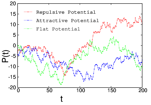
Figure 2: Time evolution of the price described by Eq. 3. Three different behavior are plotted. The red lines represents the time evolution of a RW in a repulsive quadratic potential while the blue line is in an attractive quadratic potential. The green line is the case of flat potential (simple RW). The parameters are fixed to $M=20$ and $b=\pm 1$. We can observe an over diffusion (under diffusion) in the case of repulsive (attractive) potential.

The time evolution of the “price” of such a process, is shown in Fig. 2, where we can observe three cases in which the potential is attractive, repulsive and constant (simple RW).

From this simulation, one can reconstruct the force of the process plotting $P(t+1)-P(t)$ as a function of $P(t)-P_{M}(t)$. Then, integrating from the center, one can obtain the potential.

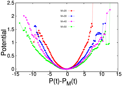
Figure 3: The plot shows the shapes of the quadratic attractive potentials defined by Eqs. 3 and  4. We can see that the amplitude of the potentials depend on the choice of the parameter $M$.

In Fig. 4 are shown the potential obtained from a simulation of the process described in Eq. 3 in the case of attractive force for various values of $M$. We can observe that the potentials have an amplitude (that is the slope of the linear force) which depends on $M$. In taka1 is shown that such a dependence can be eliminated rescaling the potential by a factor $(M-1)$.

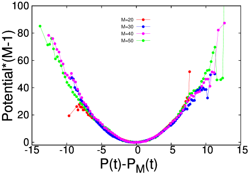
Figure 4: The different potential plotted in Fig. 3 are re-plotted scaling the potential with the factor $(M-1)$. We can see that in this way we obtain a good data collapse.

In Fig. 4 are shown the potentials plotted in Fig. 3, rescaled by the factor $(M-1)$. Indeed we can observe a good data collapse.

This idea of assuming a linear force in Eq. 3 has been tested on real data. In  taka1 a series of data from the Yen-Dollar exchange rates have been analyzed. The potential analysis for the case of the Yen-Dollar exchange rates indeed leads to the observation of rather quadratic potentials.

Anyhow, other kind of force can be considered. For example one can suppose that the price dynamic could depend only on the sign of the difference $P(t)-P_{M}(t)$. In this case an interesting model is represented by the following dynamic for a RW with only up and down steps vale1 .

$$\Bigg{\{}\begin{array}[]{ll}p(\uparrow)=1/2+\epsilon_{1}\;\;\;\mbox{for}\;\;\;P(t)-P_{M}(t)>0\\ p(\downarrow)=1/2-\epsilon_{1}\end{array}$$ (7)

$$\Bigg{\{}\begin{array}[]{ll}p(\uparrow)=1/2-\epsilon_{2}\;\;\;\mbox{for}\;\;\;P(t)-P_{M}(t)<0\\ p(\downarrow)=1/2+\epsilon_{2}\;.\end{array}$$ (10)

This model implies a tendency of destabilization (or stabilization) depending on the signs of $\epsilon_{1}$ and $\epsilon_{2}$.

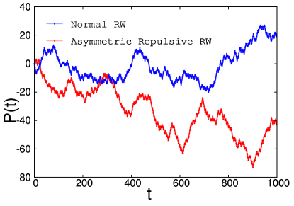
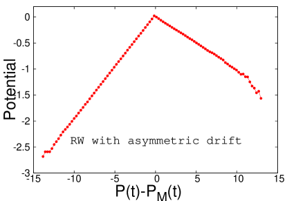
Figure 5: In figure (a) is plotted the time evolution the price whose dynamics is described by Eqs. 7 and  10, compared with the time evolution of a simple RW. In figure (b) is plotted the shape of the potential obtained analyzing the data plotted in (a). We can see a piecewise linear shape because the relative model depends only on the sign of the difference $P(t)-P_{M}(t)$. The slope of the two lines of the potential depends on the parameters $\epsilon_{1}$ and $\epsilon_{2}$.

The potential analysis for this case leads to a piecewise linear potential in which the slopes are related to $\epsilon_{1}$ and $\epsilon_{2}$. The potential will be asymmetric if $\epsilon_{1}\neq\epsilon_{2}$. In Fig. 5 and  5 are shown the time evolutions of a price whose dynamical equations is given by Eqs. 7 and  10 in the case of asymmetric repulsive potential, and the relative shape of the potential.

In order to test this model, we have considered an agent based model and we have performed the potential dynamics on the time series of the theoretical price that comes from the simulations. In the next section we are going to describe the specific rules of the agent based model we have considered.

III Application and test on an agent based model

It is instructive to analyze the effective potential scenario in agent-based models, where the price process is not defined explicitly but only through the aggregate choices of a group of traders. The simplest and most studied framework from a statistical physics perspective is that of Minority Games rev ; book1 , in which each of $N$ agents must decide at every (discrete) time step whether to buy ($a_{i}(t)=1$) or sell ($a_{i}(t)=-1$) an asset. The resulting price process is determined by the decisions of all agents through the “excess demand” $A(t)=\sum_{i=1}^{N}a_{i}(t)$. In particular, neglecting liquidity effects for the sake of simplicity, one can write that

$$P(t+1)-P(t)=A(t),$$ (11)

which amounts to defining the (log-)price as $P(t)=\sum_{t^{\prime}<t}A(t^{\prime})$.

It is clear that an agent’s trading behavior will depend on his expectations about the future price increment $A(t)$, denoted by $\mathbb{E}_{i}[A(t)]$. For example, it has been argued matteopa that if

$$\mathbb{E}_{i}[A(t)]=\psi_{i}A(t-1)+(1-\psi_{i})A(t-2),$$ (12)

agent $i$ behaves as a trend-follower for $\psi_{i}>1$ (correspondingly he perceives the market as a Majority Game with payoff $\pi_{i}(t)=a_{i}(t)A(t)$), while he behaves as a fundamentalist for $0<\psi_{i}<1$ and plays a Minority Game with payoff $\pi_{i}(t)=-a_{i}(t)A(t)$.

Let us now consider an agent who forms expectations according to (2). It is easy to see that such an agent is described by a generalization of (12). Indeed, a direct calculation shows that (2) corresponds to

$$\mathbb{E}_{i}[A(t)]\propto\sum_{\tau=1}^{M-1}\frac{M-\tau}{M}A(t-\tau).$$ (13)

Agents thus tend to discount events further back in time and give larger weight to recent price changes when estimating the future returns. Clearly, such an agent has a more complicated reaction pattern than a pure Minority or Majority Game player and will be described by a payoff function that accounts for the possibility of behaving differently in different market regimes.

Models of this type have been introduced recently and appear to be an ideal testing ground to verify the emergence of the effective potential scenario in a microscopic setting. Specifically, we have tested it on a model in which agents may switch from a trend-following to a fundamentalist attitude (and vice-versa) depending on the market conditions they perceive, which was introduced in Ref. ameno . We refer the reader to the literature for a detailed account of the model’s definition and properties. In a nutshell, it describes agents who strive to maximize the payoff

$$\pi_{i}(t)=a_{i}(t)[\mathcal{A}(t)-\epsilon\mathcal{A}(t)^{3}],$$ (14)

where $\mathcal{A}(t)=A(t)/\sqrt{N}$ is the normalized excess demand. The idea is that for small price movements ($A(t)\simeq 0$) agents perceive the game as a Majority Game as they try to identify profitable trends. However when price movements become too large, the game is perceived as a Minority Game, i.e. agents expect the price to revert to its fundamental value. As in most Minority Games, agents have fixed schemes (‘strategies’) to react to the receipt of one of $P$ possible external information patterns and learn from experience to select the strategy and, in turn, the action $a_{i}(t)$ that is more likely to deliver a positive payoff. A realistic dynamical phenomenology is obtained in a whole range of values of the model parameter $\epsilon$ when the number $N$ of players is large compared to the amount of information available to them $P$ (this is measured by a parameter $\alpha=P/N$, see ameno for details).

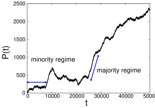
Figure 6: The time evolution of $P(t)$ for a minority-majority game with $\epsilon=1$ and $\alpha=0.05$ is shown. We can observe the alternation of different regimes. In the graph are indicated two periods by means of arrows. In the minority regime the price remains near to its fundamental value, while in the majority regime appears a well defined trend.

In Fig. 6 is shown the time evolution of $P(t)$ for a game with parameters $\alpha=0.05$ and $\epsilon=1$. This choice of parameters corresponds to be in the range in which the competition between trend followers and contrarians is stronger. In fact, in Fig. 6, we can observe some “ordered” periods, where $A(t)$ is small and well defined trends in the price dynamics appear, but also “chaotic” periods where the dynamics of the price is dominated by the contrarians. In Fig. 6 we have identified two periods in which the different behaviors of the agents are well defined and we have used these periods as dataset for our potential analysis.

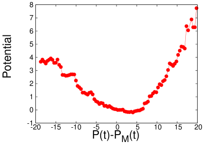
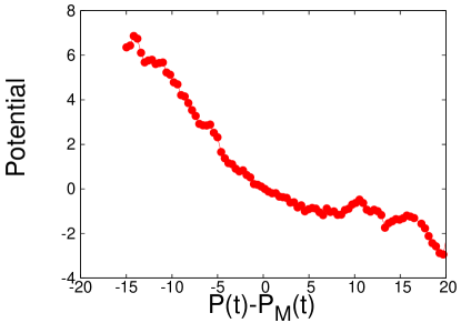
Figure 7: The potential analysis with $M=20$ for the two periods indicated in Fig. 6 is shown. The analysis for the minority region leads to an attractive (even though not really quadratic) potential. Instead, analyzing the majority region we found a repulsive potential.

In Fig. 7 are plotted the potentials obtained performing the effective potential analysis with $M=20$. We can observe that, when the market is dominated by contrarians, we obtain an attractive potential. This shape of the potential reproduce the agents’ tendency to keep the price near its “fundamental” value. We can also note that this potential is not perfectly quadratic as in model described in Eqs. 3 and  4. In fact, plotting different potentials with various values of $M$ we can not obtain a data collapse scaling the potentials with the factor $(M-1)$. In case of market dominated by trend followers, we can observe the presence of well defined trends (bubbles and crashes). In this case the agents try to follow the trends and the price tends to go away from his fundamental value. In this case we obtain a repulsive potential.

Therefore, the potential analysis is able to detect the agents’ behavior based on microscopic rules only analyzing the data of a macroscopic variable, $P(t)$.

From the viewpoint of modeling real markets, it will be very interesting to introduce an agent based model in which agents perform their decision (buy/sell) by considering their expectations about the next price increment using Eq. 13, with different constant of proportionality and different values of the ’memory’ M and not on the basis of a set of given strategies (as in the minority game framework). Work along these lines is currently in progress.

IV Results for Real Stock Prices from NYSE

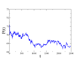
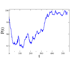
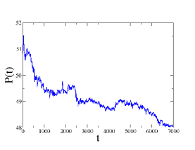
Figure 8: The time evolution of three stock index (CLF, ITU and TOL) is shown. The time is expressed in tick and correspond to one trading day.

For our potential analysis we consider as database the price time series of all the transactions of a selection of 20 NYSE stocks. These have been selected to be representative and with intermediate volatility. This corresponds to volumes of $10^{5}-10^{6}$ stocks exchanged per day. We consider 80 days from October 2004 to February 2005.

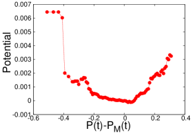
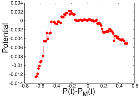
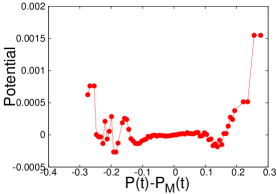
Figure 9: The effective potential method has been applied to the price evolution of the three stocks plotted in Fig. 8. We can see that the effective potential are rather asymmetric and not all quadratic. The potential in (a) seems quadratic and attractive in the central part but has asymmetric tails. The potential in (b) and (c) are not quadratic. In particular the potential in $b$ is asymmetric and looks like piecewise linear as in Fig. 5. The potential in (c) is flat like a simple RW potential.

The time series we consider are by a sequential order tick by tick. This is not identical to the price value as a function of physical time but we have tested that the results are rather insensitive to this choice.

The statistical properties of these kind of data are relatively homogeneous within the time scale of a trading day but the large jumps of the prices between different days prevent the extension of the analysis to large times vale2 . So we focus our potential analysis considering the stock-prices fluctuations within a trading day. In Fig. 8 are plotted the time evolutions of three stock indexes in a trading day.

If we perform the effective potential method for a trading day of a given stock, we found shapes of the effective potential that are very irregular and often asymmetric. In Fig 9 are plotted the results obtained for the data plotted in Fig 8. We can see that the shapes of the potentials are not always quadratic. The potential in Fig. 9 it seems rather quadratic and attractive while in Fig. 9 has a piecewise linear shape similar to the potential plotted in Fig. 5. The potential in Fig 9 seems flat as one expects from a simple RW model.

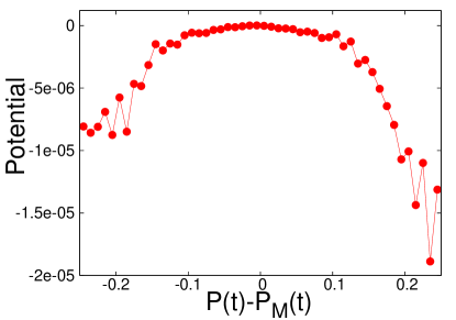
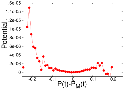
Figure 10: This plot shows the average shape of the potential over 80 trading days for two different stock indexes (BRO and PG). The shape is quite quadratic and symmetric, and in (a) is repulsive while in (b) attractive.

Instead, if we consider some average over a long period (80 trading days) of the potentials obtained for a single day, the resulting potentials seems to be quadratic as in  taka1 . In Fig. 10 are shown the average shape of the potential for two stock indexes (BRO and PG). We can observe a rather quadratic shape for the potential. In Fig. 10 the potential is quadratic and repulsive while for the index PG the potential is attractive, as we can see in Fig. 10.

References

- [1] R. N. Mantegna and H.E. Stanley. An Introduction to Econophysics: Correlation and Complexity in Finance. Cambridge University Press, New York, NY, USA, 2000.
- [2] J. P. Bouchaud and M. Potters. Theory of Financial Risk and Derivative Pricing: From Statistical Physics to Risk Management. Cambridge University Press, 2003.
- [3] V. Alfi, F. Coccetti, M. Marotta, , L. Pietronero, and M. Takayasu. Hidden forces and fluctuations from moving averages: A test study. Physica A, 2006. In printing.
- [4] M. Takayasu, T. Mizuno, and H. Takayasu. Potentials of unbalanced complex kinetics observed in market time series. 2005. E-print http://arxiv.org/abs/physics/0509020.
- [5] A. Tedeschi A. De Martino, I. Giardina and M. Marsili. Generalized minority games with adaptive trend-followers and contrarians. Phys. Rev. E 70 025104(R), 2004.
- [6] A. Cavagna. Irrelevance of memory in the minority game. Phys. Rev. E 59 R3783, 1999.
- [7] D. Challet and Y.-C. Zhang. Emergence of cooperation and organization in an evolutionary game. Physica A 246 407, 1997.
- [8] M. Marsili. Market mechanism and expectations in minority and majority games. Physica A 299 93, 2001.
- [9] V. Alfi, F. Coccetti, M. Marotta, A.Petri, and L.Pietronero. Roughness and finite size effect in the nyse stock-price fluctuations. Eur. Phys. J. B, 2006. In printing.