Quasiparticle properties in a density functional framework

Abstract

We propose a framework to construct the ground-state energy and density matrix of an $N$-electron system by solving selfconsistently a set of single-particle equations. The method can be viewed as a non-trivial extension of the Kohn-Sham scheme (which is embedded as a special case). It is based on separating the Green’s function into a quasi-particle part and a background part, and expressing only the background part as a functional of the density matrix. The calculated single-particle energies and wave functions have a clear physical interpretation as quasiparticle energies and orbitals.

I Introduction

The power of the Kohn-Sham (KS) implementation dft of density functional theory (DFT Hohen64 ) lies in its ability to incorporate complex many-body correlations (beyond Hartree-Fock) in a computational framework that is not any more difficult than the Hartree-Fock (HF) equations. In practice this means one has to solve single-particle Schrödinger equations, with local or non-local potentials, in an iterative self-consistency loop. This simplicity makes KS-DFT the only feasible approach in many modern applications of electronic structure theory. There is therefore continuing interest, not only in developing new and more accurate functionals, but also in studying conceptual improvements and extensions to the DFT framework.

The present implementations of DFT can handle short-range interelectronic correlations quite well, but often fail when dealing with near-degenerate systems characterized by a small particle-hole gap. This seems to indicate that KS-DFT does not accurately describe the Fermi surface if it deviates significantly from the noninteracting one Zha98 ; Gri00 ; Bec03 ; Gra05 ; Mol02 ; Coh01 ; Han01 . In this respect, one of the most glaring inadequacies of KS-DFT is the fact that the physically important concept of quasiparticles is missing. Even formal knowledge of the exact exchange-correlation energy functional would only lead to the total energy and the density, since the individual KS orbitals have no special significance. An exception is the HOMO orbital and energy which govern the asymptotic tail of the density. It has also been observed numerically that in exact KS-DFT the occupied single-particle energies resemble the exact ionization energies also for the deeper valence hole states Sav98 ; Cho02 ; the deviations have been analyzed theoretically in terms of a reponse contribution to the KS potential Cho02 ; Gri03 .

Quasiparticle (QP) excitations in the Landau-Migdal senseLan ; Mig form a well-known concept in many-body physics. They are most readily understood as the relics of the single-particle (s.p.) excitations in the noninteracting system when the interaction is turned on Fet71 ; Dick05 . In most electronic systems, or more generally in all normal Fermi systems, the bulk of the s.p. strength (i.e. the transition strength related to the removal or addition of a particle) is concentrated in QP states. Especially near the Fermi surface, the QP states represent the dominant physical feature and should be described properly in any appropriate single-particle theory.

The QP orbitals form a complete, linear independent, but generally nonorthogonal set. The completeness and linear independence follows from the fact that the QP states evolve from the set of single-particle eigenstates of a noninteracting Hamiltonian. Near the Fermi surface they coincide with the electron attachment states or with the dominant ionization states. Further away from the Fermi surface, QP states may acquire a width and correspond not to a single state but to a group of states in the $(N\pm 1)$-electron system characterized by rather pure one-hole or one-particle structure. The QP states have reduced s.p. strength (i.e. the normalization of the QP orbitals is less than unity). Note that QP orbitals and strengths (at least near the Fermi surface) are experimentally accessible using, e.g., electron momentum spectroscopy ems .

It is the aim of the present paper to develop formally exact single-particle equations whose solutions can be interpreted as the QP energies and orbitals, and to explore how approximations can be introduced by the modelling of small quantities in terms of functionals. The resulting formalism will be called QP-DFT and yields, apart from the QP orbitals and energies, also the total energy and the density matrix of the system.

To the best of our knowledge this is the first time such a formalism, aiming directly at the quasiparticle properties, is proposed. There are some similarities to the “correlated one-particle theory” as developed recently by Beste et al. Bes04 ; Bes05 , in that an energy-independent single-particle Hamiltonian is obtained whose eigenvalues are related to ionization energies and electron affinities. The interesting proposal in Ref. Bes04 ; Bes05 is to construct such a s.p. Hamiltonian by means of a Fock-space coupled cluster expansion, separately in the $N-1$ and $N+1$ electron system, and supplemented by a maximal overlap condition between the reference Slater determinant and the exact $N$ electron ground state (i.e. Brueckner coupled cluster). However, it is not obvious how the overcomplete set of Dyson orbitals for the $N-1$ electron system is reduced to $N$ single-particle orbitals because the technique seems to require that in general precisely $N$ exact eigenstates of the $N-1$ electron system are projected out as principal ionization states. This may be problematic in cases where the s.p. strength is fragmented, or when considering the electron gas limit. In our opinion, a general formulation should be expressed using the QP states and their associated width.

This paper is organized as follows. Sec. II reviews all necessary theoretical ingredients of the QP-DFT formalism. The natural framework for discussing QP properties is the propagator or Green’s function (GF) formulation of many-body theory Fet71 ; Dick05 . A summary of some GF results is therefore provided in Secs. II.1-II.2. See, e.g., Lin73 ; Ced77 ; Onid02 ; Ort95 ; Hol90 for reviews and general papers on the specific use of GF theory in electronic structure problems. In Sec. II.3 the standard quasiparticle concept is introduced. The fundamental equations of the new QP-DFT formalism are established in Sec. III.1. A discussion of the main properties of QP-DFT is then provided in the remainder of Sec. III, i.e. the embedding of both HF and KS-DFT, the potential exactness of the method, the asymptotic properties in coordinate space, and the electron gas limit. The final Sec. IV contains further discussion of QP-DFT (possible implementations, advantages and drawbacks), and concludes with a summary of the paper.

II Green’s function theory and the quasiparticle concept

In this section some well-established results and concepts are reviewed, in order to introduce notation and to provide an overview of the expressions needed for the QP-DFT formalism. The basic relations in GF theory can be found in many textbooks, e.g. Fet71 ; Dick05 . In Sec. II.3 the quasiparticle concept as introduced in Lan ; Mig is discussed; this material is also extensively treated in Dick05 ; Noz97 ; Mahaux .

II.1 Single-particle propagator

We initially keep the discussion as general as possible, and consider a normal (non-superconducting) Fermi system with Hamiltonian $\hat{H}=\hat{H}_{0}+\hat{V}$, where $\hat{H}_{0}$ contains the kinetic energy and external potential and $\hat{V}$ is the two-particle interaction. The s.p. propagator in the energy representation is defined as

$$G(\alpha,\beta;E)=\langle\Psi_{0}^{N}|a_{\alpha}\frac{1}{E-(\hat{H}-E_{0}^{N})+i\eta}a_{\beta}^{\dagger}+a_{\beta}^{\dagger}\frac{1}{E+(\hat{H}-E_{0}^{N})-i\eta}a_{\alpha}|\Psi_{0}^{N}\rangle$$ (1)

where $\alpha,\beta,..$ label the elements of a complete orthonormal basis set of s.p. states, the second-quantization operators $a_{\alpha}$ ($a_{\beta}^{\dagger}$) remove (add) a particle in state $\alpha$ ($\beta$), and $\eta>0$ is an infinitesimal convergence parameter. The exact ground state of the $N$-particle system is denoted by $|\Psi_{0}^{N}\rangle$ and its energy by $E_{0}^{N}$.

Inserting complete sets of eigenstates of $\hat{H}$ into Eq. (1) leads to the standard Lehmann representation of the s.p. propagator,

$$G(\alpha,\beta;E) = \sum_{n}\frac{\langle\Psi_{0}^{N}|a_{\alpha}|\Psi_{n}^{N+1}\rangle\langle\Psi_{n}^{N+1}|a_{\beta}^{\dagger}|\Psi_{0}^{N}\rangle}{E-(E_{n}^{N+1}-E_{0}^{N})+i\eta}+\sum_{n}\frac{\langle\Psi_{0}^{N}|a_{\beta}^{\dagger}|\Psi_{n}^{N-1}\rangle\langle\Psi_{n}^{N-1}|a_{\alpha}|\Psi_{0}^{N}\rangle}{E+(E_{n}^{N-1}-E_{0}^{N})-i\eta}$$ (2)

$$\equiv \sum_{n}\frac{(z_{n}^{\scriptscriptstyle(+)})_{\alpha}(z_{n}^{\scriptscriptstyle(+)})^{*}_{\beta}}{E-\epsilon^{\scriptscriptstyle(+)}_{n}+i\eta}+\sum_{n}\frac{(z_{n}^{\scriptscriptstyle(-)})_{\alpha}(z_{n}^{\scriptscriptstyle(-)})^{*}_{\beta}}{E-\epsilon^{\scriptscriptstyle(-)}_{n}-i\eta},$$

where the $|\Psi_{n}^{N\pm 1}\rangle$ are the eigenstates, and $E_{n}^{N\pm 1}$ the eigenenergies, in the $(N\pm 1)$-particle system. The notation in the last line of Eq. (2), i.e. $\epsilon^{\scriptscriptstyle(\pm)}_{n}=\pm(E_{n}^{N\pm 1}-E_{0}^{N})$ for the poles of the propagator, and

$$(z^{\scriptscriptstyle(+)}_{n})_{\alpha}=\langle\Psi_{0}^{N}|a_{\alpha}|\Psi_{n}^{N+1}\rangle;\;\;\;(z^{\scriptscriptstyle(-)}_{n})_{\alpha}=\langle\Psi_{n}^{N-1}|a_{\alpha}|\Psi_{0}^{N}\rangle$$ (3)

for the s.p. transition amplitudes, will be used throughout the paper. Note that the amplitudes $z^{\scriptscriptstyle(\pm)}_{n}$ are usually called Dyson orbitals in the electronic context.

The poles $\epsilon^{\scriptscriptstyle(+)}_{n}$ and $\epsilon^{\scriptscriptstyle(-)}_{n}$ of the propagator are located in the addition domain $(\epsilon_{0}^{\scriptscriptstyle(+)},+\infty)$ and the removal domain $(-\infty,\epsilon_{0}^{\scriptscriptstyle(-)})$, respectively. In a finite system both domains are separated by an energy interval $(\epsilon_{0}^{\scriptscriptstyle(-)},\epsilon_{0}^{\scriptscriptstyle(+)})$. The width of the interval is the particle-hole gap,

$$\epsilon_{0}^{\scriptscriptstyle(+)}-\epsilon_{0}^{\scriptscriptstyle(-)}=E^{N+1}_{0}-2E^{N}_{0}+E^{N-1}_{0}>0,$$ (4)

where positivity is guaranteed by the assumed convexity of the $E^{N}_{0}$ versus $N$ curve. Only the interval is physically relevant, but for definiteness one can take the Fermi energy as the center of the interval,

$$\epsilon_{F}=\frac{1}{2}(\epsilon_{0}^{\scriptscriptstyle(-)}+\epsilon_{0}^{\scriptscriptstyle(+)})=\frac{1}{2}(E^{N+1}_{0}-E^{N-1}_{0}).$$ (5)

In an infinite system one has $\epsilon_{0}^{\scriptscriptstyle(-)}=\epsilon_{0}^{\scriptscriptstyle(+)}=\epsilon_{F}$.

The (1-body) density matrix $[N^{\scriptscriptstyle(-)}]$ and removal energy matrix $[M^{\scriptscriptstyle(-)}]$ can be expressed in terms of the propagator as

$$N_{\alpha,\beta}^{\scriptscriptstyle(-)} \equiv \langle\Psi_{0}^{N}|a_{\beta}^{\dagger}a_{\alpha}|\Psi_{0}^{N}\rangle=\sum_{n}(z_{n}^{\scriptscriptstyle(-)})_{\alpha}(z_{n}^{\scriptscriptstyle(-)})^{*}_{\beta}=\int\frac{dE}{2\pi i}\mbox{e}^{i\eta E}G(\alpha,\beta;E),$$

$$M_{\alpha,\beta}^{\scriptscriptstyle(-)} \equiv \langle\Psi_{0}^{N}|a_{\beta}^{\dagger}[a_{\alpha},\hat{H}]|\Psi_{0}^{N}\rangle=\sum_{n}\epsilon^{\scriptscriptstyle(-)}_{n}(z_{n}^{\scriptscriptstyle(-)})_{\alpha}(z_{n}^{\scriptscriptstyle(-)})^{*}_{\beta}=\int\frac{dE}{2\pi i}\mbox{e}^{i\eta E}EG(\alpha,\beta;E).$$ (6)

The expressions in terms of the $\epsilon_{n}^{\scriptscriptstyle(-)}$ and $z^{\scriptscriptstyle(-)}_{n}$ follow by inserting the complete set of $(N-1)$-particle eigenstates of $\hat{H}$ between the $a_{\beta}^{\dagger}$ and $a_{\alpha}$ operators. The equalities on the right of Eq. (6) can then be obtained by contour integration in the complex $E$-plane, where the $\mbox{e}^{i\eta E}$ factor selects the pole contributions in the removal domain.

Any one-body observable of interest can be calculated with the density matrix. The removal energy matrix allows in addition to calculate the total energy through the Migdal-Galitskii sum rule

$$E_{0}^{N}=\frac{1}{2}\mbox{Trace}([H_{0}][N^{\scriptscriptstyle(-)}]+[M^{\scriptscriptstyle(-)}]),$$ (7)

which can be obtained by exploiting the fact that $\mbox{Trace}[M^{\scriptscriptstyle(-)}]=\langle\Psi_{0}^{N}|\hat{H}_{0}+2\hat{V}|\Psi_{0}^{N}\rangle$. The removal part of the propagator is sufficient for these purposes. However, only the (inverse of) the full propagator has a meaningful perturbative expansion, which takes the form of the Dyson equation,

$$[G(E)]^{-1}=[G_{0}(E)]^{-1}-[\Sigma(E)],$$ (8)

where $[G_{0}(E)]$ is the noninteracting propagator corresponding to the Hamiltonian $\hat{H}_{0}$ and $[\Sigma(E)]$ is the (one fermion line) irreducible selfenergy. In an ab-initio calculation, the physics input is controlled by taking a suitable approximation for the selfenergy, but here the reasoning is in terms of the exact selfenergy. The latter plays the role of an energy-dependent s.p. potential. For a discrete pole of the propagator, e.g., the amplitude obeys

$$([H_{0}]+[\Sigma(\epsilon^{\scriptscriptstyle(\pm)}_{n})])z^{\scriptscriptstyle(\pm)}_{n}=\epsilon^{\scriptscriptstyle(\pm)}_{n}z^{\scriptscriptstyle(\pm)}_{n},$$ (9)

In Fig. 1 the general diagrammatic structure of the selfenergy is shown. The two distinct types also correspond respectively to the sum of all energy-independent, and all energy-dependent, contributions to the selfenergy.

II.2 Spectral function

In general, the single-particle spectral function is related to the propagator as

$$[S(E)] = \frac{1}{2\pi i}\mbox{sign}(\epsilon_{F}-E)([G(E)]-[G(E)]^{\dagger})$$ (10)

$$= \sum_{n}(z_{n}^{\scriptscriptstyle(+)})(z_{n}^{\scriptscriptstyle(+)})^{\dagger}\delta(E-\epsilon^{\scriptscriptstyle(+)}_{n})+\sum_{n}(z_{n}^{\scriptscriptstyle(-)})(z_{n}^{\scriptscriptstyle(-)})^{\dagger}\delta(E-\epsilon^{\scriptscriptstyle(-)}_{n}).$$ (11)

The zero’th and first energy-weighted moments obey the sum rules

$$N_{\alpha,\beta} = \int_{-\infty}^{+\infty}dES(\alpha,\beta;E)=\langle\Psi_{0}^{N}|\{a_{\beta}^{\dagger},a_{\alpha}\}|\Psi_{0}^{N}\rangle$$

$$M_{\alpha,\beta} = \int_{-\infty}^{+\infty}dEES(\alpha,\beta;E)=\langle\Psi_{0}^{N}|\{a_{\beta}^{\dagger},[a_{\alpha},\hat{H}]\}|\Psi_{0}^{N}\rangle,$$ (12)

where the braces denote an anticommutator, e.g. $\{a^{\dagger}_{\beta},a_{\alpha}\}=\delta_{\alpha,\beta}$. The equalities on the right of Eq. (12) follow [similar to Eq. (6)] by inserting complete sets of eigenstates of the Hamiltonian $\hat{H}$ in both the $(N+1)$ and $(N-1)$ system,

$$\langle\Psi_{0}^{N}|\{a_{\beta}^{\dagger},[a_{\alpha},\hat{H}]\}|\Psi_{0}^{N}\rangle = \langle\Psi_{0}^{N}|a_{\beta}^{\dagger}(E_{0}^{N}-\hat{H})a_{\alpha}+a_{\alpha}(\hat{H}-E_{0}^{N})a_{\beta}^{\dagger}|\Psi_{0}^{N}\rangle$$ (13)

$$= \sum_{n}\epsilon^{\scriptscriptstyle(+)}_{n}(z_{n}^{\scriptscriptstyle(+)})(z_{n}^{\scriptscriptstyle(+)})^{\dagger}+\sum_{n}\epsilon^{\scriptscriptstyle(-)}_{n}(z_{n}^{\scriptscriptstyle(-)})(z_{n}^{\scriptscriptstyle(-)})^{\dagger}.$$

Note that the integrations in Eq. (12) are over the entire energy axis. If the integration is restricted to the removal domain $(-\infty,\epsilon_{F})$ one retrieves the one-body density matrix $[N^{\scriptscriptstyle(-)}]$ and removal energy matrix $[M^{\scriptscriptstyle(-)}]$ as defined in Eq. (6), i.e.

$$N_{\alpha,\beta}=\int_{-\infty}^{\epsilon_{F}}dES(\alpha,\beta;E)+\int_{\epsilon_{F}}^{+\infty}dES(\alpha,\beta;E)=N_{\alpha,\beta}^{\scriptscriptstyle(-)}+N_{\alpha,\beta}^{\scriptscriptstyle(+)},$$ (14)

and similarly for $M_{\alpha,\beta}=M^{\scriptscriptstyle(-)}_{\alpha,\beta}+M^{\scriptscriptstyle(+)}_{\alpha,\beta}$.

Writing the Hamiltonian as

$$\hat{H}=\sum_{\gamma\delta}\langle\gamma|H_{0}|\delta\rangle a^{\dagger}_{\gamma}a_{\delta}+\frac{1}{4}\sum_{\mu\nu\gamma\delta}\langle\mu\gamma|V|\nu\delta\rangle_{as}\,a^{\dagger}_{\mu}a^{\dagger}_{\gamma}a_{\delta}a_{\nu},$$ (15)

with

$$\langle\alpha\beta|V|\gamma\delta\rangle_{as}\equiv\langle\alpha\beta|V|\gamma\delta\rangle-\langle\alpha\beta|V|\delta\gamma\rangle$$ (16)

the antisymmetrized interaction matrix element, the (anti)commutator on the right of Eq. (12) can be worked out explicitly as

$$\{a_{\beta}^{\dagger},[a_{\alpha},\hat{H}]\}=\langle\alpha|H_{0}|\beta\rangle+\sum_{\gamma\delta}\langle\alpha\gamma|V|\beta\delta\rangle_{as}a^{\dagger}_{\gamma}a_{\delta}.$$ (17)

As a result, it is possible to express the sumrules in Eq. (12) in closed form as

$$N_{\alpha,\beta} = \delta_{\alpha,\beta}\mbox{, or }\;\;[N]=[I],$$ (18)

$$M_{\alpha,\beta} = \langle\alpha|H_{0}|\beta\rangle+\sum_{\gamma\delta}\langle\alpha\gamma|V|\beta\delta\rangle_{as}N_{\delta\gamma}^{\scriptscriptstyle(-)}\mbox{, or }\;\;[M]=[H_{0}]+[\tilde{V}_{HF}],$$ (19)

where $[I]$ is the identity matrix. These expressions will be used extensively in the following. The second term, $[\tilde{V}_{HF}]$, in Eq. (19) is the sum of all static (energy independent) selfenergy contributions, and has the form of the HF mean field, but evaluated with the exact density matrix $[N^{\scriptscriptstyle(-)}]$. A diagrammatical representation is provided by the first term in Fig. 1.

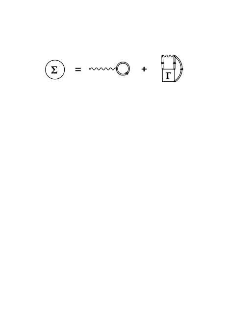
Figure 1: General structure of the exact self-energy $\Sigma(E)$ in terms of the exact 4-point vertex function $\Gamma$. The wavy line represents the antisymmetrized interaction, the double directed line is the exact propagator. The first term is the sum of all static selfenergy contributions $\tilde{V}_{HF}$, the second term involving $\Gamma$ groups all energy-dependent contributions.

II.3 Quasiparticles

In normal Fermi systems, the bulk of the spectral strength is concentrated in quasiparticle (QP) states which, in the Landau-Migdal picture, evolve adiabatically from the $N\pm 1$ eigenstates of $\hat{H}_{0}$, and can be regarded as the elementary s.p. excitations in the interacting system. In its simplest form the QP contribution to the propagator can be written as a modified noninteracting propagator,

$$G_{Q}(\alpha,\beta;E)=\sum_{j=1}^{N}\frac{(z_{Qj})_{\alpha}(z_{Qj})^{*}_{\beta}}{E-\epsilon_{Qj}-iw_{Qj}}+\sum_{j=N+1}^{\infty}\frac{(z_{Qj})_{\alpha}(z_{Qj})^{*}_{\beta}}{E-\epsilon_{Qj}+iw_{Qj}}$$ (20)

where $w_{Qj}>0$ characterizes the width of the QP excitation at energy $\epsilon_{Qj}$, and $z_{Qj}$ is the corresponding QP orbital. The first term in Eq. (20) corresponds to excitations in the $(N-1)$-particle system, as indicated by the location of the poles in the upper half-plane ($\mbox{Im}E>0$). It contains the $N$ lowest QP energies $\epsilon_{Qj}$ ($j=1,..,N$), for which $\epsilon_{Qj}<\epsilon_{F}$. The higher QP states ($j=N+1,..,\infty$) in the second term of Eq. (20) correspond to the $(N+1)$ system, as indicated by the location of the poles in the lower half-plane ($\mbox{Im}E<0$), and have $\epsilon_{Qj}>\epsilon_{F}$.

According to Eq. (10), the spectral function corresponding to the QP propagator in Eq. (20) reads

$$[S_{Q}(E)]=\sum_{j=1}^{\infty}(z_{Qj})(z_{Qj})^{\dagger}{\cal L}_{w_{Qj}}(E-\epsilon_{Qj}),$$ (21)

where the (Breit-Wigner) distribution ${\cal L}_{\Delta}(x)=\frac{\Delta/\pi}{x^{2}+\Delta^{2}}$ is normalized to unity and has width $\Delta$.

The set of QP orbitals is complete and linearly independent (in view of the 1-1 correspondence to the noninteracting system), but in general not orthogonal. The QP orbitals are different from the HF ones because of the inclusion of selfenergy contributions beyond HF (see second term in Fig. 1). This energy dependent part of the selfenergy is also responsible for a reduction of the spectroscopic strength, $z_{Qj}^{\dagger}z_{Qj}\leq 1$.

For infinite and homogenuous systems (e.g. the electron gas) the situation is particularly transparant, since all matrix quantities are diagonal in a plane-wave basis, and reduce to continuous functions of s.p. momentum $p$. For momenta close to the Fermi momentum ($p\approx p_{F}$) the QP energy is the solution of $\epsilon_{Q}(p)=p^{2}/(2m)+\mbox{Re}\Sigma(p;\epsilon_{Q}(p))$, and coincides with the Fermi energy at $p_{F}$, i.e. $\epsilon_{Q}(p_{F})=\epsilon_{F}$. The spectral function $S(p;E)$ is dominated by a sharp QP peak at $\epsilon_{Q}(p)$, having a width $w_{Q}(p)$. The width $w_{Q}(p)$ is proportional to $\mbox{Im}\Sigma(p;\epsilon_{Q}(p))$ and vanishes for $p\rightarrow p_{F}$. While the QP excitations are only unambiguously defined near the Fermi surface, the concept can be extended to all momenta.

Similar considerations also apply to finite systems, where the QP excitation corresponds to a state or group of states having rather pure s.p. character. The $(N\pm 1)$-particle states near the Fermi energy (where no poles of the selfenergy are present) are usually characterized by spectroscopic factors of the order of (but smaller than) unity. In closed-shell atoms, e.g., the first ionization state $\Psi_{0}^{N-1}$ (corresponding to the first pole in the removal domain of the propagator) typically has a spectroscopic factor of about 95% Neck01 . In that case the QP orbital in Eq. (20) coincides with the Dyson orbital. More deeply bound orbitals may acquire a width, but have similar summed strength concentrated near an average QP energy. The QP orbital in Eq. (20) is then representative for the transition amplitudes to these states.

The QP contribution to the sumrules in Eq. (12) is given by

$$[N_{Q}]=\sum_{j=1}^{\infty}z_{Qj}z_{Qj}^{\dagger};\;\;\;[M_{Q}]=\sum_{j=1}^{\infty}\epsilon_{Qj}z_{Qj}z_{Qj}^{\dagger}.$$ (22)

Note that the QP width does not contribute to the $0^{\mbox{th}}$ and $1^{\mbox{st}}$ moment, and drops out from all subsequent considerations.

Finally, it should be noted that the simple ansatz in Eq. (20) does not provide a valid description of a QP excitation $j$ far away from the QP energy $\epsilon_{Qj}$. The energy-dependence in Eq. (21) can then be slightly misleading, as the tails of the Breit-Wigner distribution extend beyond the Fermi energy. In reality the strength of a QP excitation either belongs to the $N-1$ or to the $N+1$ system. The QP contribution to the separate $[N^{\scriptscriptstyle(\pm)}]$ and $[M^{\scriptscriptstyle(\pm)}]$ should therefore not be determined directly by Eqs. (14,21), but rather by the location of the poles in the lower or upper halfplane, i.e.

$$[N_{Q}^{\scriptscriptstyle(-)}] = \int\frac{dE}{2\pi i}\mbox{e}^{i\eta E}[G_{Q}(E)]=\sum_{j=1}^{N}z_{Qj}z_{Qj}^{\dagger}$$

$$\mbox{}[M_{Q}^{\scriptscriptstyle(-)}] = \int\frac{dE}{2\pi i}\mbox{e}^{i\eta E}E[G_{Q}(E)]=\sum_{j=1}^{N}\epsilon_{Qj}z_{Qj}z_{Qj}^{\dagger},$$ (23)

and similarly for

$$[N_{Q}^{\scriptscriptstyle(+)}]=\sum_{j=N+1}^{\infty}z_{Qj}z_{Qj}^{\dagger};\;\;\;[M_{Q}^{\scriptscriptstyle(+)}]=\sum_{j=N+1}^{\infty}\epsilon_{Qj}z_{Qj}z_{Qj}^{\dagger}.$$ (24)

III Quasiparticle equations

III.1 Derivation of the QP-DFT equations

For the following it is important to realize that, given arbitrary hermitian matrices $[N_{Q}]$ and $[M_{Q}]$ with $[N_{Q}]$ positive-definite, one can always write the unique decomposition of Eq. (22). This can be achieved by constructing the unique basis that solves the (generalized) eigenvalue problem

$$[M_{Q}]u_{j}=\lambda_{j}[N_{Q}]u_{j};\;\;\;\;u_{j}^{\dagger}[N_{Q}]u_{k}=\delta_{j,k},$$ (25)

where $[N_{Q}]$ plays the role of a metric matrix; the QP energies and orbitals given by $\epsilon_{Qj}=\lambda_{j}$ and $z_{Qj}=[N_{Q}]u_{j}$ then fulfill Eq. (22).

The eigenvalue problem in Eq. (25) can be considered as a set of s.p. equations determining the QP orbitals and energies. We now rewrite the unknown operators $[N_{Q}]$ and $[M_{Q}]$ in a more useful form that suggests possible approximation schemes.

Since the QP contribution to the spectral function is dominant, it makes sense to isolate it,

$$[S(E)]=[S_{Q}(E)]+[S_{B}(E)],$$ (26)

and concentrate on the residual small ’background’ contribution $[S_{B}(E)]$. In fact, the full energy dependence of $[S_{B}(E)]$ is not needed, since one can apply the quasiparticle-background separation of Eq. (26) to the zero’th and first energy-weighted moments as well, i.e. one has

$$[N]=[N_{Q}]+[N_{B}];\;\;\;[M]=[M_{Q}]+[M_{B}],$$ (27)

where the total energy integrals $[N_{B}]=[N_{B}^{\scriptscriptstyle(-)}]+[N_{B}^{\scriptscriptstyle(+)}]$ and $[M_{B}]=[M_{B}^{\scriptscriptstyle(-)}]+[M_{B}^{\scriptscriptstyle(+)}]$ can again be split in a removal and addition part. Note that the matrices $[N]$ and $[M]$ on the left side of Eq. (27) are known in closed form through Eqs. (18-19), so it follows that

$$[N_{Q}] = [I]-[N_{B}],$$ (28)

$$\mbox{}[M_{Q}] = [H_{0}]+[\tilde{V}_{HF}]-[M_{B}].$$ (29)

One then arrives at the remarkable conclusion that modelling the background contributions $[M_{B}^{\scriptscriptstyle(\pm)}]$ and $[N_{B}^{\scriptscriptstyle(\pm)}]$ as a functional of e.g. the density matrix $[N^{\scriptscriptstyle(-)}]$, is sufficient to generate a selfconsistent set of s.p. equations. Using Eqs. (28-29) the eigenvalue problem in Eq. (25) can be expressed as

$$([H_{0}]+[\tilde{V}_{HF}\{N^{\scriptscriptstyle(-)}\}]-[M_{B}\{N^{\scriptscriptstyle(-)}\}])u_{j}=\lambda_{j}([I]-[N_{B}\{N^{\scriptscriptstyle(-)}\}])u_{j},$$ (30)

where the functional dependency of $[M_{B}]$ and $[N_{B}]$ is indicated between braces. Note that also the HF-like potential $[\tilde{V}_{HF}]$ is by definition [see Eq. (19)] expressed in terms of the density matrix, as indicated in Eq. (30).

Having an initial estimate for $[N^{\scriptscriptstyle(-)}]$ allows to construct the matrices $[N_{B}]$ and $[M_{B}]$, as well as the HF-like potential $[\tilde{V}_{HF}]$. The eigenvalue problem in Eq. (30) can now be solved, yielding QP energies $\epsilon_{Qj}=\lambda_{j}$ and orbitals $z_{Qj}=([I]-[N_{B}\{N^{\scriptscriptstyle(-)}\}])u_{j}$. The $N$ solutions with lowest energy represent excitations in the $N-1$ system, and should be used to update the density matrix $[N^{\scriptscriptstyle(-)}]=[N_{Q}^{\scriptscriptstyle(-)}]+[N_{B}^{\scriptscriptstyle(-)}]$,

$$[N^{\scriptscriptstyle(-)}_{\mbox{\small new}}]=\sum_{j=1}^{N}z_{Qj}z_{Qj}^{\dagger}+[N_{B}^{\scriptscriptstyle(-)}\{N^{\scriptscriptstyle(-)}\}].$$ (31)

This closes the selfconsistency loop, which can be iterated to convergence. The total energy then follows from Eq. (7),

$$E_{0}^{N}=\frac{1}{2}\sum_{j=1}^{N}z^{\dagger}_{Qj}([H_{0}]+\epsilon_{Qj})z_{Qj}+\frac{1}{2}\mbox{Trace}\left([H_{0}][N^{\scriptscriptstyle(-)}_{B}\{N^{\scriptscriptstyle(-)}\}]+[M_{B}^{\scriptscriptstyle(-)}\{N^{\scriptscriptstyle(-)}\}]\right).$$ (32)

The above formalism, henceforth called quasiparticle DFT (QP-DFT), generates the total energy, the density matrix, and the individual QP energies and orbitals, starting from a model for the background contributions $[M_{B}^{\scriptscriptstyle(\pm)}]$ and $[N_{B}^{\scriptscriptstyle(\pm)}]$ as a functional of the density matrix. It is intuitively clear that this is a reasonable strategy: the external potential appears directly in the QP hamiltonian $[M]-[M_{B}]$ through the $[H_{0}]$ term of Eq. (19), and primarily influences the position of the QP peaks. One may then assume the background part to be generated by ’universal’ electron-electron correlations, and to be a good candidate for modelling. Equation (30), determining the QP energies and orbitals, is the central result of the present paper, and its properties will now be discussed in detail.

III.2 HF and KS-DFT as special cases of QP-DFT

We first show that both HF and KS-DFT theory are included in the general QP-DFT treatment.

For HF this is rather obviously achieved by setting all background quantities $[M_{B}^{\scriptscriptstyle(\pm)}]$ and $[N_{B}^{\scriptscriptstyle(\pm)}]$ equal to zero in Eq. (30). Since the metric matrix on the right of Eq. (30) is now simply the identity matrix, one has $z_{Qj}=u_{j}$ and the QP orbitals form an orthonormal set obeying $([H_{0}]+[\tilde{V}_{HF}])z_{Qj}=\epsilon_{Qj}z_{Qj}$. The matrix $[\tilde{V}_{HF}]$ is given by Eq. (19) where the density matrix $[N^{\scriptscriptstyle(-)}]$ in the present approximation follows from Eq. (31) with $[N^{\scriptscriptstyle(-)}_{B}]=0$, i.e.

$$[N^{\scriptscriptstyle(-)}]=\sum_{j=1}^{N}z_{Qj}z_{Qj}^{\dagger}.$$ (33)

One can see that $[M]=[H_{0}]+[\tilde{V}_{HF}]$ is just the ordinary HF hamiltonian, and the total energy obtained from Eq. (32) by setting $[N_{B}^{\scriptscriptstyle(-)}]=[M_{B}^{\scriptscriptstyle(-)}]=0$,

$$E_{0}^{N}=\frac{1}{2}\sum_{j=1}^{N}(z_{Qj}^{\dagger}[H_{0}]z_{Qj}+\epsilon_{Qj})$$ (34)

is equivalent to the HF total energy.

The KS-DFT case is somewhat more difficult, but one also starts by setting $[N_{B}^{\scriptscriptstyle(\pm)}]=0$ in Eq. (30), so the QP states $z_{Qj}$ form an orthonormal set obeying

$$([H_{0}]+[\tilde{V}_{H}]+[\tilde{V}_{F}]-[M_{B}])z_{Qj}=\epsilon_{Qj}z_{Qj}.$$ (35)

Here the HF-like potential has been split into its direct and exchange components, $[\tilde{V}_{HF}]=[\tilde{V}_{H}]+[\tilde{V}_{F}]$. As the density matrix is again given by Eq. (33), both components only receive contributions from the occupied ($j=1,..,N$) orbitals $z_{Qj}$:

$$(\tilde{V}_{H})_{\alpha,\beta} = \mbox{ }\sum_{\gamma\delta}\langle\alpha\gamma|V|\beta\delta\rangle\sum_{j=1}^{N}(z_{Qj})_{\delta}(z_{Qj})^{*}_{\gamma},$$

$$(\tilde{V}_{F})_{\alpha,\beta} = \mbox{}-\sum_{\gamma\delta}\langle\alpha\gamma|V|\delta\beta\rangle\sum_{j=1}^{N}(z_{Qj})_{\delta}(z_{Qj})^{*}_{\gamma}.$$ (36)

For the Coulomb interaction and taking as s.p. labels for the electrons the space coordinate and (third component of) spin, $\alpha\equiv{\bf r}m_{s}$ , this reduces to the familiar expression

$$\tilde{V}_{H}({\bf r}m_{s},{\bf r}^{\prime}m^{\prime}_{s})+\tilde{V}_{F}({\bf r}m_{s},{\bf r}^{\prime}m^{\prime}_{s})=\delta_{m_{s},m^{\prime}_{s}}\delta({\bf r}-{\bf r}^{\prime})\sum_{j=1}^{N}\sum_{m^{\prime\prime}_{s}}\int d{\bf r}^{\prime\prime}\frac{|z_{Qj}({\bf r}^{\prime\prime}m^{\prime\prime}_{s})|^{2}}{|{\bf r}-{\bf r}^{\prime\prime}|}-\sum_{j=1}^{N}\frac{z_{Qj}({\bf r}m_{s})z^{*}_{Qj}({\bf r}^{\prime}m^{\prime}_{s})}{|{\bf r}-{\bf r}^{\prime}|}.$$ (37)

Note that for compactness we continue to employ the general matrix notation used so far, with the understanding that sums over s.p. labels should be replaced by coordinate space integrations where appropriate. The total energy follows from Eq. (32) with $[N^{\scriptscriptstyle(\pm)}_{B}]=0$,

$$E_{0}^{N}=\frac{1}{2}\sum_{j=1}^{N}(z_{Qj}^{\dagger}[H_{0}]z_{Qj}+\epsilon_{Qj})+\frac{1}{2}\mbox{Trace}[M_{B}^{\scriptscriptstyle(-)}].$$ (38)

The unknown $[M^{\scriptscriptstyle(\pm)}_{B}]$ should now be determined by identification with the results of a KS-DFT calculation.

We allow explicit dependence on the KS orbitals $\varphi_{KSj}$, and write the exchange-correlation energy functional as

$$E_{xc}=\sum_{j=1}^{N}\varphi_{KSj}^{\dagger}[\epsilon_{xc}]\varphi_{KSj}.$$ (39)

Specializing e.g. to a hybrid functional (the derivation for a functional with general orbital dependencies proceeds in a similar fashion) with a fraction $\beta$ of exact exchange, the matrix $[\epsilon_{xc}]$ in coordinate-spin space reads,

$$\epsilon_{xc}({\bf r}\,m_{s},{\bf r}^{\prime}\,m^{\prime}_{s})=-\frac{\beta}{2}\sum_{j=1}^{N}\frac{\varphi_{KSj}({\bf r}\,m_{s})\varphi_{KSj}^{*}({\bf r}^{\prime}\,m^{\prime}_{s})}{|{\bf r}-{\bf r}^{\prime}|}+\delta_{m_{s},m^{\prime}_{s}}\delta({\bf r}-{\bf r}^{\prime})f_{\beta}(\rho({\bf r}),\nabla\rho({\bf r})),$$ (40)

where the second term contains a local functional of the electron density $\rho({\bf r})$ and its gradient (assuming for simplicity a spin-saturated system). The corresponding exchange-correlation potential $[V_{xc}]$, appearing in the KS equation, then reads

$$V_{xc}({\bf r}\,m_{s},{\bf r}^{\prime}\,m^{\prime}_{s})=-\beta\sum_{j=1}^{N}\frac{\varphi_{KSj}({\bf r}\,m_{s})\varphi_{KSj}^{*}({\bf r}^{\prime}\,m^{\prime}_{s})}{|{\bf r}-{\bf r}^{\prime}|}+\delta_{m_{s},m^{\prime}_{s}}\delta({\bf r}-{\bf r}^{\prime})\{f_{\beta}+\rho\frac{\partial f_{\beta}}{\partial\rho}-\nabla\cdot(\rho\frac{\partial f_{\beta}}{\partial\nabla\rho})\}.$$ (41)

Identification of the orbitals and energies in the KS equation

$$([H_{0}]+[V_{H}]+[V_{xc}])\varphi_{KSj}=\epsilon_{KSj}\varphi_{KSj}$$ (42)

with those in Eq. (35) then requires

$$[M_{B}]=[V_{F}]-[V_{xc}].$$ (43)

Identification of the KS total energy

$$E_{0}^{N} = \sum_{j=1}^{N}\varphi_{KSj}^{\dagger}([H_{0}]+[V_{H}])\varphi_{KSj}+E_{xc}$$ (44)

$$= \frac{1}{2}\sum_{j=1}^{N}(\varphi_{KSj}^{\dagger}[H_{0}]\varphi_{KSj}+\epsilon_{KSj})+E_{xc}-\frac{1}{2}\sum_{j=1}^{N}\varphi_{KSj}^{\dagger}[V_{xc}]\varphi_{KSj}$$

with Eq. (38) requires

$$\mbox{Trace}[M_{B}^{\scriptscriptstyle(-)}]=\sum_{j=1}^{N}\varphi_{KSj}^{\dagger}(2[\epsilon_{xc}]-[V_{xc}])\varphi_{KSj}.$$ (45)

Choosing the $[M_{B}^{\scriptscriptstyle(\pm)}]$ operators as

$$[M_{B}^{\scriptscriptstyle(-)}]=[P](2[\epsilon_{xc}]-[V_{xc}])[P];\;\;\;[M_{B}^{\scriptscriptstyle(+)}]=[V_{F}]-[V_{xc}]-[P](2[\epsilon_{xc}]-[V_{xc}])[P],$$ (46)

where $[P]=\sum_{j=1}^{N}z_{Qj}z_{Qj}^{\dagger}$ projects onto the occupied QP orbitals, fulfills the requirements of both Eq. (43) and of Eq. (45); this choice therefore leads to the same results as the KS-DFT approximation, for the total energy as well as the orbitals and orbital energies.

One concludes that the QP-DFT formulation is flexible enough to reproduce HF or KS-DFT results by specific choices of $[N_{B}^{\scriptscriptstyle(\pm)}]$ and $[M_{B}^{\scriptscriptstyle(\pm)}]$. Note that the KS-DFT formalism is embedded in a slightly tortuous way, as $[N_{B}^{\scriptscriptstyle(\pm)}]=0$ would normally imply the absence of a background contribution to the first-order moment $[M_{B}^{\scriptscriptstyle(\pm)}]$ as well. A similar situation is encountered in Brueckner-Hartree-Fock theoryBHF , in which the real part of the selfenergy causes a shift in the QP energy, but the corresponding reduction of strength through the imaginary part of the selfenergy is neglected.

III.3 Potential exactness

It should be clear that GF quantities like the propagator, spectral function, or selfenergy, are well-defined and can in principle be calculated exactly. Also the separation of the spectral strength into QP and background parts can be performed for any system. In fact, defining the QP part can usually be done in several ways which are all, however, equivalent at the Fermi surface. Note that the density matrix and the total energy only contain the $0^{\mbox{th}}$ and $1^{\mbox{st}}$ energy-weighted moment $[N^{\scriptscriptstyle(-)}]$ and $[M^{\scriptscriptstyle(-)}]$, and do not depend on the QP-background separation. As long as one sticks to one unique prescription, the QP orbitals and energies are well-defined quantities, and so are the background contributions $[N_{B}^{\scriptscriptstyle(\pm)}]$ and $[M_{B}^{\scriptscriptstyle(\pm)}]$. The fundamental expressions in Eq. (30-32) are therefore always valid.

As an example of an unambiguous definition of QP excitations one can e.g., in the spirit of Landau-Migdal theory, consider the lowest order expansion of the selfenergy around $\epsilon_{F}$:

$$[\Sigma(E)]=[\Sigma(\epsilon_{F})]+(E-\epsilon_{F})[\Sigma^{\prime}(\epsilon_{F})],$$ (47)

where $[\Sigma^{\prime}(E)]$ is the first derivative of the selfenergy with respect to energy. For infinite homogenuous systems the right side of Eq. (47) is a real function, since $\mbox{Im}\Sigma(p,E)=\frac{\partial}{\partial E}\mbox{Im}\Sigma(p,E)=0$ at the Fermi energy $E=\epsilon_{F}$. In a finite system the right of Eq. (47) is an hermitian matrix, since $[\Sigma(E)]=[\Sigma(E)]^{\dagger}$ in a finite pole-free interval around the Fermi energy. Substituting the linearized selfenergy (47) into Eq. (9) leads to

$$([H_{0}]+[\Sigma(\epsilon_{F})]-\epsilon_{F}[\Sigma^{\prime}(\epsilon_{F})])u=E([I]-[\Sigma^{\prime}(\epsilon_{F})])u,$$ (48)

defining the QP excitations. Note the formal similarity to Eq. (30), and the fact that the metric matrix is positive-definite as $[\Sigma^{\prime}(\epsilon_{F})]$ is a negative-definite hermitian matrix. While Eq. (48) results in a correct description for $E\approx\epsilon_{F}$, it may not be appropriate away from the Fermi surface, when the linear approximation (47) breaks down.

It should be stressed that the possibility of defining QP excitations in various ways is not a shortcoming of the present approach, but rather a reflection of the physical reality that QP excitations are only unambiguously defined near the Fermi surface, where the density of states in the $N\pm 1$ system is small. The complete description of the s.p. properties in an interacting many-body system is contained in the energy dependence of the spectral function. Any effective s.p. Hamiltonian can at most describe the peaks in the spectral function, i.e. identify the energy regions where the s.p. strength is concentrated and assign an average transition amplitude to this region.

Finally we should explain the use of the density matrix as the independent variable for the functional modelling of $[N_{B}^{\scriptscriptstyle(\pm)}]$ and $[M_{B}^{\scriptscriptstyle(\pm)}]$ in Eq. (30). In the present context it seems most natural to do this in terms of a matrix quantity. Moreover, for the class of systems with fixed two-body interaction $\hat{V}$ and varying nonlocal external potentials (i.e. varying $\hat{H}_{0}$), the fundamental theorem of density matrix functional theory dmft implies that all quantities can be expressed as functionals of the density matrix. This holds in particular for the $[N_{B}^{\scriptscriptstyle(\pm)}]$ and $[M_{B}^{\scriptscriptstyle(\pm)}]$, once a unique prescription is agreed upon.

It is of course also possible to consider the electron density $\rho$ as the basic variable, provided one restricts oneself to the class of systems with local external potentials. In that case one is again formally assured of the existence of functionals for all quantities. Note that the functional in Sec. III.2 reproducing the KS-DFT results, even when the exact KS functional is used, is not the exact QP-DFT functional since it does not yield the correct density matrix; the exact QP-DFT functional would definitely have $[N_{B}^{\scriptscriptstyle(\pm)}]\neq 0$.

III.4 Asymptotics in coordinate space for finite systems

For notational convenience the spin dependence is dropped here. In coordinate space the background quantities $N_{B}^{\scriptscriptstyle(-)}({\bf r},{\bf r}^{\prime})$ and $M_{B}^{\scriptscriptstyle(-)}({\bf r},{\bf r}^{\prime})$ represent nonlocal operators, as they have a finite trace. The complete background operators $N_{B}({\bf r},{\bf r}^{\prime})$ and $M_{B}({\bf r},{\bf r}^{\prime})$ can be local or nonlocal.

It seems plausible that the background operators are short-ranged in the sense that correlation effects should become insignificant at large distances. I.e. the limit $|{\bf r}|\rightarrow\infty$ of the background operators should drop out when considering the asymptotic behavior of the quasiparticles in Eq. (30). This requires for $|{\bf r}|\rightarrow\infty$ that

$$|\int d{\bf r}^{\prime}N_{B}({\bf r},{\bf r}^{\prime})z({\bf r}^{\prime})|/|z({\bf r})|\rightarrow 0$$ (49)

for an arbitrary s.p. orbital $z({\bf r})$. It is sufficient to take $[N_{B}]$ local and asymptotically vanishing, but nonlocal implementations are also possible. For $[M_{B}]$ one requires that for $|{\bf r}|\rightarrow\infty$,

$$M_{B}({\bf r},{\bf r}^{\prime})\rightarrow-\frac{N_{B}^{\scriptscriptstyle(-)}({\bf r},{\bf r}^{\prime})}{|{\bf r}-{\bf r}^{\prime}|}+H_{B}({\bf r},{\bf r}^{\prime})$$ (50)

where $H_{B}({\bf r},{\bf r}^{\prime})$ is again short-ranged in the sense of Eq. (49). Note that one does not require $[N_{B}^{\scriptscriptstyle(-)}]$ to be short-ranged, but its contribution to the Fock term in $[\tilde{V}_{HF}\{N^{\scriptscriptstyle(-)}\}]$ of Eq. (30) should be canceled by $[M_{B}]$ in the limit $|{\bf r}|\rightarrow\infty$. The $[N_{B}^{\scriptscriptstyle(-)}]$ contribution to the Hartree term remains, since this is not affected when taking the limit $|{\bf r}|\rightarrow\infty$ in Eq. (30).

With the characteristics (49-50) of the exact QP-DFT functional, the background operators simply drop out of the asymptotic behavior of Eq. (30), and one is left with (for an external charge $Z$)

$$\left(-\frac{\nabla^{2}}{2m}-\frac{Z-N}{r}-\epsilon_{Qi}\right)z_{Qi}({\bf r})-\sum_{j=1}^{N}z_{Qj}({\bf r})\int\frac{d{\bf r^{\prime}}}{|{\bf r}-{\bf r}^{\prime}|}z^{*}_{Qj}({\bf r}^{\prime})u_{i}({\bf r}^{\prime})=0.$$ (51)

Note that, for $|{\bf r}|\rightarrow\infty$, one has $z_{Qi}({\bf r})=u_{i}({\bf r})$ since the metric matrix $[I]-[N_{B}]$ becomes the identity by virtue of Eq. (49). The Hartree term gives rise to the $N/r$ potential, and only the Fock term built with the $N$ lowest QP orbitals needs further analysis. In fact, one immediately sees that the behavior of the Fock term is the same as the one studied in Ref. Handy (or more generally in Ref. Kat80 ). The asymptotic expansion

$$\frac{1}{{|{\bf r}-{\bf r}^{\prime}|}}=\frac{1}{r}+\sum_{L=1}^{\infty}\frac{r^{\prime L}}{r^{L+1}}P_{L}(\mbox{cos}\omega),$$ (52)

where $P_{L}$ is a Legendre polynomial and $\omega$ the angle between ${\bf r}$ and ${\bf r}^{\prime}$, can be substituted in the Fock term of Eq. (51). The first ($L=0$) term in Eq. (52) then only contributes in case of removal-type ($i=1,..,N$) QP orbitals, since [see Eq. (25)]

$$\int d{\bf r^{\prime}}\,z^{*}_{Qj}({\bf r}^{\prime})u_{i}({\bf r}^{\prime})=z^{\dagger}_{Qj}u_{i}=u^{\dagger}_{j}[N_{Q}]u_{i}=\delta_{i,j},$$ (53)

and effectively changes the asymptotic charge to $Z-N+1$. A similar analysis as in Ref. Kat80 then proves that the removal QP orbital with the slowest decay is the HOMO one ($i=N$), and goes like $\sim\mbox{e}^{-\alpha r}r^{\beta}$ with $\alpha^{2}=-2\epsilon_{QN}$ and $\beta=(Z-N+1)/\alpha$. The Fock term imposes the same exponential decay (except in very special cases) on the other removal QP orbitals, but with an accompanying power law that decreases faster by at least $1/r^{2}$.

For the addition-type ($i=N+1,..,+\infty$) QP orbitals the first term in Eq. (52) does not contribute to the Fock term in Eq. (51), and the asymptotic charge remains $Z-N$. This means that for neutral atoms no Rydberg sequence of bound addition-type QP orbitals is present, which is in agreement with the real physical situation. Also note that, unlike HF, the presence of the $[M_{B}]$ term in Eq. (30) does allow for the possibility that some addition-type QP orbitals become bound for neutral systems. The asymptotics of the bound addition-type QP orbitals is again correct, with an exponential decay governed by their individual separation energies $\epsilon_{Qi}$. They go like $\sim\mbox{e}^{-\alpha r}r^{\beta}$ with $\alpha^{2}=-2\epsilon_{Qi}$ and $\beta=(Z-N)/\alpha$; the Fock term in Eq. (51) cannot influence this, since all removal-type QP orbitals decay faster.

III.5 The electron gas limit

We consider for simplicity the spin-unpolarized electron gas at density $\rho$, and suppress the spin indices. To find the electron gas limit of the $[M^{\scriptscriptstyle(\pm)}_{B}]$ and $[N^{\scriptscriptstyle(\pm)}_{B}]$ quantities one needs the momentum distribution $n(p)$ and the removal energy $r(p)$, defined as

$$n(p)=\langle\Psi_{0}|a^{\dagger}_{\bf p}a_{\bf p}|\Psi_{0}\rangle;\;\;r(p)=\langle\Psi_{0}|a^{\dagger}_{\bf p}[a_{\bf p},\hat{H}]|\Psi_{0}\rangle.$$ (54)

The QP-background separation can be made once a QP spectrum $\epsilon_{Q}(p)$ and strength $Z_{Q}(p)$ is defined. Near the Fermi surface the standard definitions

$$\epsilon_{Q}(p)=p^{2}/(2m)+\mbox{Re}\Sigma(p;\epsilon_{Q}(p));\;\;\;Z_{Q}(p)=1/(1-\frac{\partial\mbox{Re}\Sigma(p;E)}{\partial E})_{E=\epsilon_{Q}(p)}$$ (55)

are valid. For momenta far from $p_{F}$ Eq. (55) may break down, e.g. the equation defining $\epsilon_{Q}(p)$ may have multiple roots, or the strength $Z_{Q}(p)$ may become larger than unity. An alternative definition, valid for all momenta, must then be used. For an example of such a procedure we refer to Dewu05 , where the QP-background separation was made in the context of a $GW$ description Hed65 ; vB&H of the electron gas.

The background quantities in the electron gas are now expressed as

$$N^{\scriptscriptstyle(-)}_{B}(p) = n(p)-\theta(p_{F}-p)Z_{Q}(p);\;\;\;N^{\scriptscriptstyle(+)}_{B}(p)=1-n(p)-\theta(p-p_{F})Z_{Q}(p)$$

$$M^{\scriptscriptstyle(-)}_{B}(p) = r(p)-\theta(p_{F}-p)Z_{Q}(p)\epsilon_{Q}(p);\;\;\;M^{\scriptscriptstyle(+)}_{B}(p)=p^{2}/(2m)+\tilde{V}_{F}(p)-r(p)-\theta(p-p_{F})Z_{Q}(p)\epsilon_{Q}(p),$$ (56)

where $\tilde{V}_{F}(p)$ is the Fock-like potential (evaluated with the exact momentum distribution $n(p)$). The typical behavior of these background quantities as a function of momentum can be found in Fig. 1 of Ref.Dewu05 .

For the purpose of applying the electron gas results to inhomogenuous systems, it is not a priori clear what the equivalent of the Local Density Approximation would be. Working with the Wigner transform would seem the most straightforward,

$$N_{B}^{\scriptscriptstyle(-)}({\bf r}\,m_{s},{\bf r}^{\prime}\,m^{\prime}_{s}) = \delta_{m_{s},m^{\prime}_{s}}\left.\int\frac{d{\bf p}}{(2\pi)^{3}}\mbox{e}^{i{\bf p}\cdot({\bf r}-{\bf r}^{\prime})}N^{\scriptscriptstyle(-)}_{B}(p)\right|_{\rho=\rho({\bf R})},$$ (57)

but there are several possibilities which reduce to the same electron gas result in the homogenuous limit.

IV Summary and discussion

The concept of quasiparticles is an important tool to understand and describe normal Fermi systems. In this paper we developed a set of single-particle equations whose solutions correspond to the QP orbitals and energies. When the residual small background contributions are expressed as universal functionals of the density or density matrix, a single-particle selfconsistency problem (the QP-DFT scheme) is generated that can be easily solved for an approximate choice of the functionals.

The QP-DFT scheme would seem to offer many advantages as compared to KS-DFT. There is no need for the difference between the kinetic energy of the interacting systems and a reference system. All s.p. orbitals and energies have physical meaning, in contrast to the KS orbitals. The asymptotic behavior of the QP orbitals comes out correct, provided the background operators are short-ranged. On the down side: since we no longer have a sharp Fermi surface, particle-number conservation is not automatically guaranteed, and should be built into the functionals.

The fact that KS-DFT is built in as a special case is a very important feature of QP-DFT. In a sense, one cannot do worse than KS-DFT, since one adds more parameters to the model. Moreover, the new parameters are truly new degrees of freedom (the introduction of the metric matrix, allowing a softening of the Fermi surface), which cannot be mimicked by taking a more sophisticated KS functional.

The modelling of the background operators $[N_{B}^{\scriptscriptstyle(\pm)}]$, $[M_{B}^{\scriptscriptstyle(\pm)}]$ is basically virgin territory. One option would be to exploit the relation (46) with the KS formalism, using an existing XC functional form for $[M_{B}^{\scriptscriptstyle(\pm)}]$, adding a similar form for $[N_{B}^{\scriptscriptstyle(\pm)}]$, and (re)parametrize by fitting to total energies and ionization energies in a training set of atoms and molecules.

Alternatively, one could devise parametrizations by performing GF calculations on a series of test systems, and construct the background operators directly from the calculated spectral function. A step in this direction was taken in Ref. g0w0 , where we applied an ab-initio selfenergy of the $G_{0}W_{0}$ type to a series of closed-shell atoms. The QP-DFT scheme outlined in the present paper was used in first iteration (no selfconsistency) to generate the first-order corrections to the HF picture. We then constructed a simple QP-DFT functional that depends only on HF quantities, but was able to reproduce the most important results of the underlying ab-initio model.

References

• (1) W. Kohn and L.J. Sham, Phys. Rev. 140, A1133 (1965)
• (2) P. Hohenberg and W. Kohn, Phys. Rev. 136, B864 (1964)
• (3) Y. Zhang, W. Yang, J. Chem. Phys. 109, 2604 (1998)
• (4) O.V. Gritsenko, B. Ensing, P.R.T. Schipper, E.J. Baerends, J. Phys. Chem. A 104, 8558 (2000)
• (5) A.D. Becke, J. Chem. Phys. 119, 2972 (2003)
• (6) J. Grafenstein, D. Cremer, Mol. Phys. 103, 279 (2005)
• (7) K. Molawi, A.J. Cohen, N.C. Handy, Int. J. Quantum Chem. 89, 86 (2002)
• (8) A.J. Cohen, N.C. Handy, Mol. Phys. 99, 607 (2001)
• (9) N.C. Handy, A.J. Cohen, Mol. Phys. 99, 403 (2001)
• (10) A. Savin, C.J. Umrigar, X. Gonze, Chem. Phys. Lett. 288, 391 (1998)
• (11) D.P. Chong, O.V. Gritsenko, E.J. Baerends, J. Chem. Phys. 116, 1760 (2002)
• (12) O.V. Gritsenko, B. Braida, E.J. Baerends, J. Chem. Phys. 119, 1937 (2003)
• (13) L.D. Landau, JETP 3, 920 (1957); JETP 5, 101 (1957); JETP 8, 70 (1959)
• (14) A.B. Migdal, Theory of Finite Fermi Systems and Applications to Atomic Nuclei (John Wiley and sons, New York, 1967)
• (15) A.L. Fetter and J.D. Walecka, Quantum Theory of Many Particle Systems (McGraw-Hill, New York, 1971)
• (16) W.H. Dickhoff and D. Van Neck, Many-Body Theory Exposed: propagator description of many particle quantum mechanics (World Scientific, Singapore, 2005)
• (17) E. Weigold and I.E. McCarthy, Electron Momentum Spectroscopy (Kluwer Academic/Plenum Publishers, New York, 1999)
• (18) A. Beste and R.J. Bartlett, J. Chem. Phys. 120, 8395 (2004)
• (19) A. Beste and R.J. Bartlett, J. Chem. Phys. 123, 154103 (2005)
• (20) J.V. Ortiz, J. Chem. Phys. 103, 5630 (1995)
• (21) J. Linderberg and Y. Oehrn, Propagators in Quantum Chemistry (Academic, London, 1973)
• (22) L.S. Cederbaum and W. Domcke, Adv. Chem. Phys. 36, 205 (1977)
• (23) G. Onida, L. Reining and A. Rubio, Rev. Mod. Phys. 74, 601 (2002)
• (24) L.J. Holleboom and J.G. Snijders, J. Chem. Phys. 93, 5826 (1990)
• (25) P. Nozières, Theory of Interacting Fermi Systems (Addison-Wesley, Reading, Massachusetts, 1997)
• (26) C. Mahaux and R. Sartor, Adv. Nucl. Phys. 20, 1 (1991)
• (27) D. Van Neck, K. Peirs and M. Waroquier, J. Chem. Phys. 115, 4095 (2001)
• (28) K.A. Brueckner and C.A. Levinson, Phys. Rev. 97, 1344 (1955)
• (29) T.L. Gilbert, Phys. Rev. B 12, 2111 (1975)
• (30) J. Katriel and E.R. Davidson, Proc. Natl. Acad. Sci. USA, Vol.70, 4403 (1980)
• (31) N.C. Handy, M.T. Marron and H.J. Silverstone, Phys. Rev. 180, 45 (1969)
• (32) Y. Dewulf, D. Van Neck and M. Waroquier, Phys. Rev. B 71, 245122 (2005)
• (33) L. Hedin, Phys. Rev. 139, A796 (1965)
• (34) U. von Barth and B. Holm, Phys. Rev. B 54, 8411 (1996); B. Holm and U. von Barth, Phys. Rev. B 57, 2108 (1998); B. Holm, Phys. Rev. Lett. 83, 788 (1999)
• (35) S. Verdonck, D. Van Neck, P.W. Ayers and M. Waroquier, to be published.