Stochastic volatility of financial markets as the fluctuating rate of trading:
an empirical study

Abstract

We present an empirical study of the subordination hypothesis for a stochastic time series of a stock price. The fluctuating rate of trading is identified with the stochastic variance of the stock price, as in the continuous-time random walk (CTRW) framework. The probability distribution of the stock price changes (log-returns) for a given number of trades $N$ is found to be approximately Gaussian. The probability distribution of $N$ for a given time interval $\Delta t$ is non-Poissonian and has an exponential tail for large $N$ and a sharp cutoff for small $N$. Combining these two distributions produces a nontrivial distribution of log-returns for a given time interval $\Delta t$, which has exponential tails and a Gaussian central part, in agreement with empirical observations.

Introduction: stochastic volatility, subordination, and fluctuations in the number of trades.

The stock price $S_{t}$ is a stochastic series in time $t$. It is commonly characterized by the probability distribution $P_{\Delta t}(x)$ of detrended log-returns $x=\ln(S_{t_{2}}/S_{t_{1}})-\mu\Delta t$, where the time interval $\Delta t=t_{2}-t_{1}$ is called the time lag or time horizon, and $\mu$ is the average growth rate. For a simple multiplicative (geometric) random walk, the probability distribution is Gaussian: $P_{\Delta t}(x)\propto\exp(-x^{2}/2v\Delta t)$, where $v=\sigma^{2}$ is the variance, and $\sigma$ is the volatility. However, the empirically observed probability distribution of log-returns is not Gaussian. It is well known that the distribution has power-law tails for large $x$ Stanley99b ; Stanley99a . However, the distribution is also non-Gaussian for small and moderate $x$, where it follows the tent-shaped exponential (also called double-exponential) Laplace law: $P_{\Delta t}(x)\propto\exp(-c|x|/\sqrt{\Delta t})$, as emphasized in Ref. Silva04 . The exponential distribution was found by many researchers Bouchaud ; Miranda01 ; McCauley03 ; Kaizoji04 ; Remer04 ; Makowiec04 ; Matia04 ; Vicente06 , so it should be treated as a ubiquitous stylized fact for financial markets Silva04 .

In order to explain the non-Gaussian character of the distribution of returns, models with stochastic volatility were proposed in literature Praetz72 ; Hull87 ; Heston93 ; Sircar-book . If the variance $v_{t}$ changes in time, then $v\Delta t$ in the Gaussian distribution should be replaced by the integrated variance $V_{\Delta t}=\int_{t_{1}}^{t_{2}}v_{t}\,dt$. If the variance is stochastic, then we should average over the probability distribution $Q_{\Delta t}(V)$ of the integrated variance $V$ for the time interval $\Delta t$:

$$P_{\Delta t}(x)=\int_{0}^{\infty}dV\,\frac{e^{-x^{2}/2V}}{\sqrt{2\pi V}}\,Q_{\Delta t}(V).$$ (1)

The representation (1) is called the subordination Feller-book ; Clark73 . In this approach, the non-Gaussian character of $P_{\Delta t}(x)$ results from a non-trivial distribution $Q_{\Delta t}(V)$.

In the models with stochastic volatility, the variables $v$ or $V$ are treated as hidden stochastic variables. One may try to identify these phenomenological variables with some empirically observable and measurable components of the financial data. It was argued Mandelbrot67 ; Ane00 ; Stanley00 that the integrated variance $V_{\Delta t}$ may correspond to the number of trades (transactions) $N_{\Delta t}$ during the time interval $\Delta t$: $V_{\Delta t}=\xi N_{\Delta t}$, where $\xi$ is a coefficient volume . Every transaction may change the price up or down, so the probability distribution $P_{N}(x)$ after $N$ trades would be Gaussian:

$$P_{N}(x)=\frac{e^{-x^{2}/2\xi N}}{\sqrt{2\pi\xi N}}.$$ (2)

Then, the subordinated representation (1) becomes

$$P_{\Delta t}(x)=\int_{0}^{\infty}dN\,\frac{e^{-x^{2}/2\xi N}}{\sqrt{2\pi\xi N}}\,K_{\Delta t}(N),$$ (3)

where $K_{\Delta t}(N)$ is the probability to have $N$ trades during the time interval $\Delta t$. (We assume that $N$ is large and use integration, rather than summartion, over $N$.) In this approach, the stochastic variance $v$ reflects the fluctuating rate of trading in the market.

Performing the Fourier transform of (3) with respect to $x$, we find that the characteristic function $\tilde{P}_{\Delta t}(k_{x})$ is directly related to the Laplace transform $\tilde{K}_{\Delta t}(k_{N})$ of $K_{\Delta t}(N)$ with respect to $N$, where $k_{x}$ and $k_{N}$ are the Fourier and Laplace variables conjugated to $x$ and $N$:

$$\tilde{P}_{\Delta t}(k_{x})=\int\limits_{0}^{\infty}dNe^{-N\xi k_{x}^{2}/2}K_{\Delta t}(N)=\tilde{K}_{\Delta t}(\xi k_{x}^{2}/2).$$ (4)

In this paper, we study whether the subordinated representation (3) agrees with financial data. First, we verify whether $P_{N}(x)$ is Gaussian, as suggested by Eq. (2). Second, we check whether empirical data satisfy Eq. (4). Third, we obtain $K_{\Delta t}(N)$ empirically and, finally, discuss whether $P_{\Delta t}(x)$ constructed from Eq. (3) agrees with the data. Refs. Ane00 ; Stanley00 have already presented evidence in favor of the first conjecture; however, the other questions were not studied systematically in literature.

The subordination was also studied in physics literature as the continuous-time random walk (CTRW) Montroll65 ; Montroll84 . Refs. Scalas00 ; Sabatelli02 ; Masoliver03 focused on the probability distribution of the waiting time $\Delta t$ between two consequtive transactions ($\Delta N=1$). Our approach is to study the distribution function $K_{\Delta t}(N)$, which gives complementary information and can be examined for a wide variety of time lags. In Ref. Dremin05 , this function was studied for some Russian stocks.

We use the TAQ database from NYSE TAQ , which records every transaction in the market (tick-by-tick data). We focus on the Intel stock (INTC), because it is highly traded, with the average number of transactions per day about $2.5\times 10^{4}$. Here we present the data for the period 1 January – 31 December 1999, but we found similar results for 1997 as well Silva-thesis . Because of difficulties in dealing with overnight price changes, we limit our consideration to the intraday data. Since $\Delta t$ is relatively short here, the term $\mu\Delta t$ is small and can be neglected.

Probability distribution of log-returns $x$ after $N$ trades.

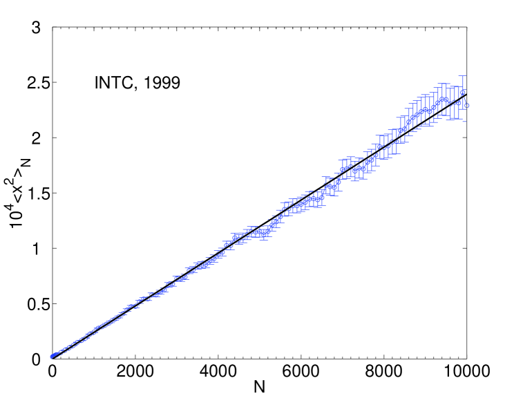
Figure 1: The variance of log-returns $\langle x^{2}\rangle_{N}$ after $N$ trades plotted vs. $N$.

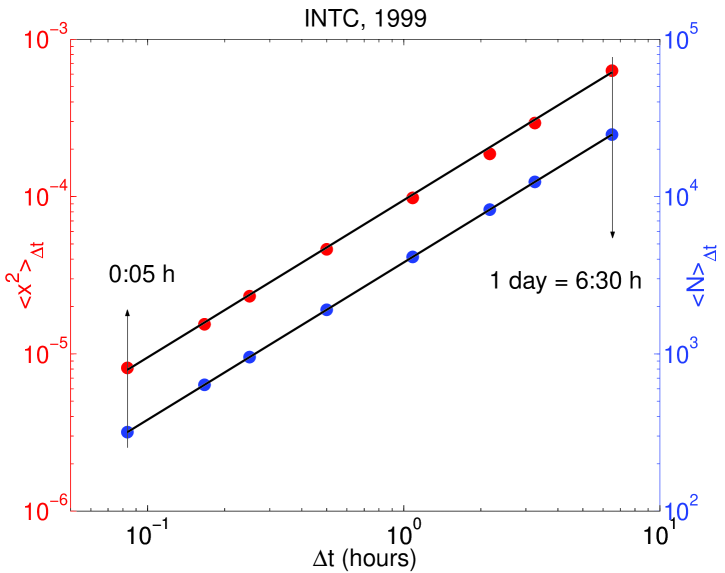
Figure 2: The variance of log-returns $\langle x^{2}\rangle_{\Delta t}$ (upper points, left scale) and the average number of trades $\langle N\rangle_{\Delta t}$ (lower points, right scale) vs. the time lag $\Delta t$. The solid lines of slope 1 represent the proportionality relations (5).

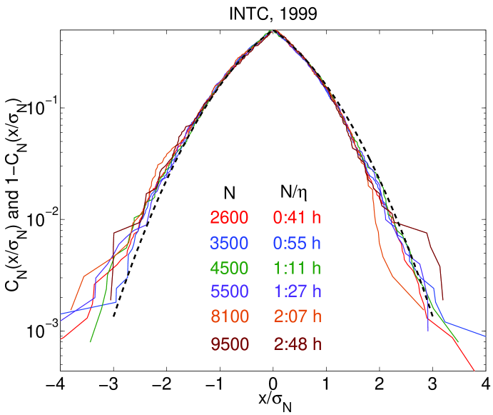
Figure 3: Cumulative distribution $C_{N}(x/\sigma_{N})$ of normalized log-returns after $N$ trades, where $\sigma_{N}^{2}=\langle x^{2}\rangle_{N}$, compared with the Gaussian distribution (dashed curve). $N/\eta$ is the typical time interval between $N$ trades.

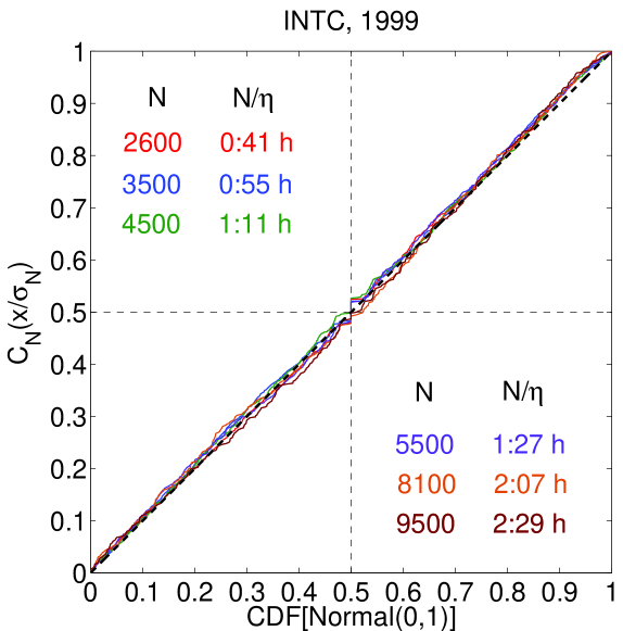
Figure 4: The parametric Q-Q plot of the empirical cumulative distribution $C_{N}(x/\sigma_{N})$ of normalized log-returns vs. the Gaussian distribution for the parameter $x$ from $-\infty$ to $+\infty$.

It follows from Eq. (2) that $\langle x^{2}\rangle_{N}=\xi N$, where $\langle x^{2}\rangle_{N}$ is the second moment of $x$ after $N$ trades. It is also natural to expect that the average number of trades $\langle N\rangle_{\Delta t}$ during the time interval $\Delta t$ is proportional to $\Delta t$ with some coefficient $\eta$. Thus, we expect

$$\langle x^{2}\rangle_{N}=\xi N,\;\langle N\rangle_{\Delta t}=\eta\Delta t,\;\langle x^{2}\rangle_{\Delta t}=\theta\Delta t,\;\theta=\xi\eta.$$ (5)

Notice that the coefficient $\theta=\langle v\rangle$ is the mean variance. Figs. 1 and 2 show that the relations (5) are indeed satisfied. We extract the values of the coefficients from the slopes of these plots: $\xi=2.4\times 10^{-8}$ per one trade, $\eta=3.8\times 10^{3}$ trades/hour, and $\theta=9.5\times 10^{-5}$ per hour. The relation $\theta=\xi\eta$ is satisfied only approximately, but within the measurement accuracy.

In Figs. 3 and 4, we examine the empirical probability distribution $P_{N}(x)$ of log-returns $x$ after $N$ trades. In Fig. 3, the cumulative distribution functions $C_{N}(x)=\int_{-\infty}^{x}dx^{\prime}P_{N}(x^{\prime})$ for $x<0$ and $1-C_{N}(x)$ for $x<0$ are compared with the Gaussian distribution shown by the dashed line. The log-return $x$ is normalized by $\sigma_{N}=\sqrt{\langle x^{2}\rangle_{N}}$. The empirical distributions $P_{N}(x)$ for different $N$ agree with the Gaussian in the central part, but there are deviations in the tails, as expected for large $|x|$. Similar results were found in Fig. 6 of Ref. Farmer05 .

Fig. 4 shows the Q-Q plot similar to the one constructed in Ref. Ane00 . This is a parametric plot, where the vertical axis shows the empirical $C_{N}(x/\sigma_{N})$, and the horizontal axis shows the cumulative Gaussian distribution of $x/\sigma$, whereas the parameter $x$ changes from $-\infty$ to $+\infty$. The plots for different $N$ are all close to the diagonal, which indicates agreement between the empirical and the Gaussian distribution functions. Fig. 4 emphasizes the central part of the distribution, whereas Fig. 3 emphasizes the tails. Overall, we conclude the empirical distribution $P_{N}(x)$ is reasonably close to the Gaussian in the central part, so Eq. (2) is approximately satisfied.

When the time lag approaches one day, the number of data points become too small to construct reliable probability densities, so we cannot verify the Gaussian hypothesis beyond the intraday data. When the time lag is too short, and the corresponding $N$ is small, the log-returns are discrete and cannot be described by a continuous function, such as Gaussian. We found that the distribution of $x$ becomes reasonably smooth only after a thousand of trades Silva-thesis . Discreteness of the distribution for small $N$ can be seen in Fig. 11 of Ref. Farmer04 .

The characteristic function for log-returns and the Laplace transform for the number of trades.

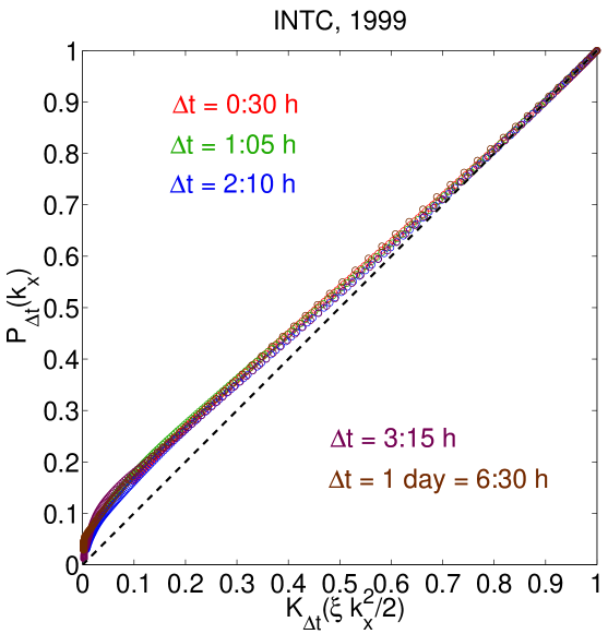
Figure 5: The parametric plot of the Fourier transform $\tilde{P}_{\Delta t}(k_{x})$ vs. the Laplace transform $\tilde{K}_{\Delta t}(\xi k_{x}^{2}/2)$ verifying Eq. (4) for the parameter $k_{x}$ from $-\infty$ to $+\infty$.

The subordination hypothesis (3) can be examined further by checking the relation (4) between the Fourier transform $\tilde{P}_{\Delta t}(k_{x})$ for log-returns and the Laplace transform $\tilde{K}_{\Delta t}(k_{N})$ for the number of trades. These functions can be directly constructed from the data. As shown in Ref. Silva04 , $\tilde{P}_{\Delta t}(k_{x})\approx(1/n)\sum_{j=1}^{n}e^{ik_{x}x_{j}}$ and $\tilde{K}_{\Delta t}(k_{N})\approx(1/m)\sum_{l=1}^{m}e^{-k_{N}N_{l}}$, where the sums are taken over all occurrences of the log-returns $x_{j}$ and the numbers of trades $N_{l}$ during a time interval $\Delta t$ in a dataset. Because the frequency of appearances of a given $x_{j}$ or $N_{l}$ is proportional to the corresponding probability density, these sums approximate the integral definitions $\tilde{P}_{\Delta t}(k_{x})=\int_{-\infty}^{+\infty}dx\,e^{ik_{x}x}P_{\Delta t}(x)$ and $\tilde{K}_{\Delta t}(k_{N})=\int_{0}^{\infty}dN\,e^{-k_{N}N}K_{\Delta t}(N)$.

In Fig. 5, we show the parametric plot of $\tilde{P}_{\Delta t}(k_{x})$ vs. $\tilde{K}_{\Delta t}(\xi k_{x}^{2}/2)$. The vertical axis shows $\tilde{P}_{\Delta t}(k_{x})$, and the horizontal axis shows $\tilde{K}_{\Delta t}(\xi k_{x}^{2}/2)$, whereas the parameter $k_{x}$ changes from from $-\infty$ to $+\infty$. The upper right corner $(1,1)$ corresponds to $k_{x}=0$, and the lower left corner $(0,0)$ corresponds to large $|k_{x}|$. The parameter $\xi$ used in Fig. 5 is extracted from the slope of $\langle x^{2}\rangle_{N}$ vs. $N$ in Fig. 1. The relations

$$\left.\frac{d^{2}\tilde{P}_{\Delta t}(k_{x})}{dk_{x}^{2}}\right|_{k_{x}=0}=-\langle x^{2}\rangle_{\Delta t},\>\left.\frac{d\tilde{K}_{\Delta t}(k_{N})}{dk_{N}}\right|_{k_{N}=0}=-\langle N\rangle_{\Delta t}$$ (6)

and Eq. (5) ensure that the slope of the parametric plot near the point $(1,1)$ corresponds to the diagonal. Overall, the plots for different $\Delta t$ in Fig. 5 are close to the diagonal, but deviate in the lower corner for large $|k_{x}|$, which indicates that the subordination relation (4) is satisfied only approximately. Notice that no assumptions about the functional form of $K_{\Delta t}(N)$ are made in Eq. (4). The only assumption is that $P_{N}(x)$ is Gaussian (2), and the distributions of $x$ and $N$ are uncorrelated, so they can be combined in Eq. (3).

Probability distribution of the number of trades $N$ during the time interval $\Delta t$.

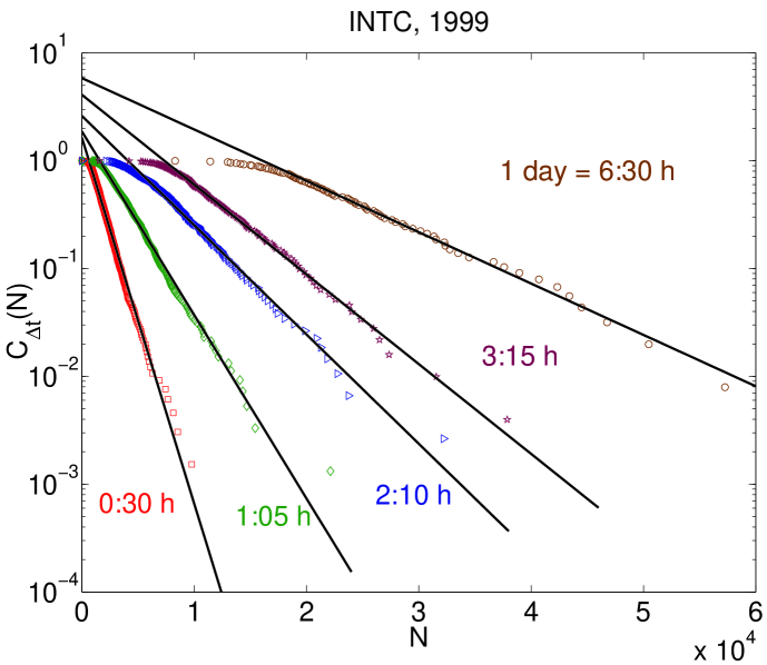
Figure 6: Empirical cumulative distribution $C_{\Delta t}(N)$ for the number of trades $N$ during the time interval $\Delta t$, plotted in the log-linear scale. The solid lines illustrate exponential tails.

Fig. 6 shows the log-linear plot of the empirically constructed cumulative distribution $C_{\Delta t}(N)=\int_{N}^{\infty}K_{\Delta t}(N^{\prime})\,dN^{\prime}$ for the number of trades $N$ during the time interval $\Delta t$. The straight lines are eye guides, which indicate that the probability distributions $K_{\Delta t}(N)$ are exponential for large $N$. The slopes of the lines are related to $\langle N\rangle_{\Delta t}=\eta\Delta t$, so we can approximate $K_{\Delta t}(N)\propto\exp(-N/\eta\Delta t)$ for large $N$. For small $N$, Fig. 6 shows that $C_{\Delta t}(N)$ is flat and $K_{\Delta t}(N)$ is suppressed, so that $K_{\Delta t}(N=0)=0$. It is indeed very improbable to have no trades at all for an extended time period $\Delta t$. For long enough $\Delta t$, we expect that $K_{\Delta t}(N)$ would become a Gaussian function of $N$ centered at $\langle N\rangle_{\Delta t}=\eta\Delta t$. However, this regime has not been achieved yet for the time lags $\Delta t$ shown in Fig. 6. For short $\Delta t$, we also found that $\langle N^{2}\rangle_{\Delta t}\propto\langle N\rangle^{2}_{\Delta t}$ with a coefficient somewhat smaller than 2, as expected for an approximately exponential distribution.

Notice that the exponential behavior of the empirical $K_{\Delta t}(N)$ shown in Fig. 6 is inconsistent with the Poisson distribution $K_{\Delta t}^{\rm Poisson}(N)=e^{-\eta\Delta t}(\eta\Delta t)^{N}/N!$ expected for trades occurring randomly and independently at the average rate $\eta$. It was suggested in literature that $K_{\Delta t}(N)$ may be approximated by the log-normal or gamma distributions. We do not attempt to discriminate between the alternative hypotheses here, but sometimes these functions may look alike Banerjee06 . A qualitatively similar distribution $K_{\Delta t}(N)$ was found for some Russian stocks in Ref. Dremin05 .

Probability distribution of log-returns $x$ after the time interval $\Delta t$.

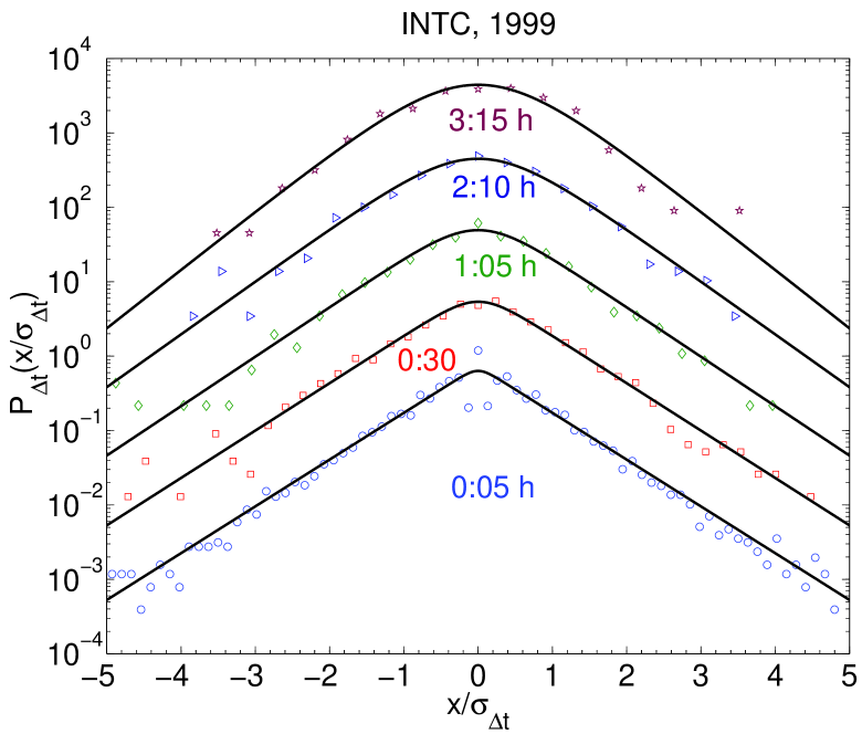
Figure 7: Probability density $P_{\Delta t}(x/\sigma_{\Delta t})$ of normalized log-returns after the time lag $\Delta t$, where $\sigma_{\Delta t}^{2}=\langle x^{2}\rangle_{\Delta t}$. The solid lines are fits to the Heston model with $1/\gamma=50$ min. The curves are offset vertically by the factors of 10.

Having established that $P_{N}(x)$ is approximately Gaussian (2), and $K_{\Delta t}(N)$ is approximately exponential for short $\Delta t$, we can obtain $P_{\Delta t}(x)$ from Eq. (3). Substituting these expressions into Eq. (3), we get

$$P_{\Delta t}(x)\approx\int_{0}^{\infty}dN\,\frac{e^{-x^{2}/2\xi N}}{\sqrt{2\pi\xi N}}\,\frac{e^{-N/\eta\Delta t}}{\eta\Delta t}=\frac{e^{-|x|\sqrt{2/\theta\Delta t}}}{\sqrt{2\theta\Delta t}}.$$ (7)

Eq. (7) shows that the exponential distribution of the number of trades $N$ results in the exponential (Laplace) distribution of log-returns $x$. This can be understood as follows. The integral (7) can be taken exactly, but one can also evaluate it approximately by integrating around the optimal value of $N_{*}=|x|\sqrt{\eta\Delta t/2\xi}$ that minimizes the negative expression in the exponent of Eq. (7) and maximizes the integrand. We see that the probability to have a given log-return $x$ is controlled by the probability to have the optimal number of trades $N_{*}(x)$. Thus, the distribution $P_{\Delta t}(x)$ has the fatter (exponential) tails than Gaussian, because the probability to have a large $x$ is enhanced by fluctuations with large $N$.

On the other hand, for very small $x$, the optimal value $N_{*}$ becomes limited by the cutoff in $K_{\Delta t}(N)$ for small $N$. At this point, the optimal value $N_{*}$ stops depending on $x$, so $P_{\Delta t}(x)$ becomes Gaussian. Thus, we expect to see the Gaussian behavior in $P_{\Delta t}(x)$ for small $|x|$ and the exponential behavior for medium and large $|x|$. Fig. 7 shows a log-linear plot of the empirical probability density $P_{\Delta t}(x)$. In agreement with the qualitative analysis presented above, we observe that the data points follow the parabolic (Gaussian) curve for small $|x|$ and fall on the straight (exponential) lines for large $|x|$. The range of $x$ occupied by the Gaussian expands when the time lag $\Delta t$ increases, because the cutoff in $K_{\Delta t}(N)$ for small $N$ increases with the increase of $\Delta t$, as shown in Fig. 6. We conclude that the subordination hypothesis (3) is qualitatively valid, and, particularly, it explains the exponential distribution $P_{\Delta t}(x)$ for $x$ as a result of the exponential distribution $K_{\Delta t}(N)$ for the number of trades $N$.

The solid lines in Fig. 7 show fits of the data to the Heston model. The Heston model Heston93 is a model with stochastic volatility, which has the advantage of being exactly solvable. A closed-form solution for $P_{\Delta t}(x)$ was obtained in Ref. Dragulescu02 , and Fig. 7 shows fits of the data to the formula derived there. Refs. Silva04 ; Dragulescu02 pointed out that $P_{\Delta t}(x)$ in the Heston model has the exponential tails and Gaussian center, in qualitative and quantitative agreement with the empirical distribution of log-returns. Given the verification of the subordination hypothesis presented in this paper, one may ask whether the Heston model describes the probability distribution $K_{\Delta t}(N)$ for the number of trades $N$. A detailed study of this question will be presented in a separate paper U-shape .

We also would like to point out that Eq. (7) represents a special case of the variance-gamma distribution introduced by Madan and Seneta Madan90 . The Heston model solution Dragulescu02 reduces to the variance-gamma distribution in the limit of short $\Delta t$, see Eqs. (48) and (49) in Ref. Dragulescu02 .

References

- (1) P. Gopikrishnan, V. Plerou, L. A. N. Amaral, M. Meyer, and H. E. Stanley, Phys. Rev. E 60, 5305 (1999).
- (2) V. Plerou, P. Gopikrishnan, L. A. N. Amaral, M. Meyer, and H. E. Stanley, Phys. Rev. E 60, 6519 (1999).
- (3) A. C. Silva, R. E. Prange, and V. M. Yakovenko, Physica A 344, 227 (2004).
- (4) J.-P. Bouchaud and M. Potters, Theory of Financial Risks (Cambridge University Press, Cambridge, 2000).
- (5) L. C. Miranda and R. Riera, Physica A 297, 509 (2001).
- (6) J. L. McCauley and G. H. Gunaratne, Physica A 329, 178 (2003).
- (7) T. Kaizoji, Physica A 343, 662 (2004).
- (8) R. Remer and R. Mahnke, Physica A 344, 236 (2004).
- (9) D. Makowiec, Physica A 344, 36 (2004).
- (10) K. Matia, M. Pal, H. Salunkay, and H. E. Stanley, Europhys. Lett. 66, 909 (2004).
- (11) R. Vicente, C. M. de Toledo, V. B. P. Leite, and N. Caticha, Physica A 361, 272 (2006).
- (12) P. D. Praetz, The Journal of Business 45, 49 (1972).
- (13) J. Hull and A. White, The Journal of Finance 42, 281 (1987).
- (14) S. L. Heston, Review of Financial Studies 6, 327 (1993).
- (15) J. P. Fouque, G. Papanicolaou, and K. R. Sircar, Derivatives in Financial Markets with Stochastic Volatility (Cambridge University Press, Cambridge, 2000).
- (16) W. Feller, An Introduction to Probability Theory and Its Applications (Wiley, New York, 1971), Vol. II.
- (17) P. K. Clark, Econometrica 41, 135 (1973).
- (18) B. Mandelbrot and H. M. Taylor, Operations Research 15, 1057 (1967).
- (19) T. Ané and H. Geman, The Journal of Finance 55, 2259 (2000).
- (20) V. Plerou, P. Gopikrishnan, L. A. N. Amaral, X. Gabaix, and H. E. Stanley, Phys. Rev. E 62, R3023 (2000).
- (21) One may also consider the volume of trades instead of the number of trades. In that case, empirical analysis is technically more complicated, so we limit our consideration to the number of trades.
- (22) E. W. Montroll and G. H. Weiss, J. Math. Phys. 6, 167 (1965).
- (23) E. W. Montroll and M. F. Shlesinger, in Nonequilibrium Phenomena II: From Stochastics to Hydrodynamics, edited by J. L. Lebowitz and E. W. Montroll (North-Holland, Amsterdam, 1984).
- (24) F. Mainardi, M. Raberto, R. Gorenflo and E. Scalas, Physica A 287, 468 (2000).
- (25) L. Sabatelli, S. Keating, J. Dudley, and P. Richmond, Eur. Phys. J. B 27, 273 (2002).
- (26) J. Masoliver, M. Montero, and G. H. Weiss, Phys. Rev. E 67, 021112 (2003).
- (27) I. M. Dremin and A. V. Leonidov, Physica A 353, 388 (2005).
- (28) NYSE data, http://www.nysedata.com/.
- (29) A. C. Silva, Ph.D. Thesis, Ch. 5 (University of Maryland, 2005), http://arxiv.org/abs/physics/0507022.
- (30) L. Gillemot, J. D. Farmer, F. Lillo, http://arxiv.org/abs/physics/0510007.
- (31) J. D. Farmer, L. Gillemot,, F. Lillo, S. Mike, A. Sen, Quantitative Finance 4, 383 (2004).
- (32) A. Banerjee, V. M. Yakovenko, and T. Di Matteo, Physica A 370, 5459 (2006).
- (33) A. Drăgulescu and V. M. Yakovenko, Quantitative Finance 2, 443 (2002).
- (34) We are also aware that the variation of volatility during a day has the well-known U-shape, with the highest number of trades at the opening and closing times Silva-thesis .
- (35) D. B. Madan and E. Seneta, The Journal of Business 63, 511 (1990).