Auxiliary-field quantum Monte Carlo study of first- and second-row post-d elements

Abstract

A series of calculations for the first- and second-row post-d elements (Ga-Br and In-I) are presented using the phaseless auxiliary-field quantum Monte Carlo (AF QMC) method. This method is formulated in a Hilbert space defined by any chosen one-particle basis, and maps the many-body problem into a linear combination of independent-particle solutions with external auxiliary fields. The phase/sign problem is handled approximately by the phaseless formalism using a trial wave function, which in our calculations was chosen to be the Hartree-Fock solution. We used the consistent correlated basis sets of Peterson and coworkers, which employ a small core relativistic pseudopotential. The AF QMC results are compared with experiment and with those from density-functional (GGA and B3LYP) and coupled-cluster CCSD(T) calculations. The AF QMC total energies agree with CCSD(T) to within a few milli-hartrees across the systems and over several basis sets. The calculated atomic electron affinities, ionization energies, and spectroscopic properties of dimers are, at large basis sets, in excellent agreement with experiment.

I Introduction

We recently extended the phaseless auxiliary-field quantum Monte Carlo (AF QMC) approach zhang_krakauer to any single-particle basis, and applied it to the study of molecular systems with Gaussian basis sets gafqmc . The calculated all-electron total energies of many first-row atoms and molecules at their equilibrium geometries show typical systematic errors of no more than a few milli-hartrees (mE_h) compared to exact results. This is roughly comparable to that of CCSD(T), coupled-cluster with single and double excitations plus an approximate treatment of triple excitations. For stretched bonds in H₂O gafqmc as well as N₂ and F₂ gafqmc2 , the phaseless AF QMC exhibits better overall accuracy and a more uniform behavior than CCSD(T) in mapping the potential energy curve.

In this paper, we apply the new method to heavier systems and present a systematic study of several properties of the first- and second-row post-d elements (Ga-Br and In-I). Our goal is to systematically benchmark the new method in different environments and to compare it to experiment, as well as to a high level correlation method such as CCSD(T).

Throughout this work, we used the consistent correlated basis sets of Peterson and co-workers, which were introduced recently for the first-, second-, and third-row non-transition metal post-d elements peterson1 ; peterson2 . These are denoted by cc-pVnZ-PP (with $n=$ D, T, Q, 5) basis_sets_web , and systematically converge to the complete basis set limit much like the correlation consistent basis sets of Dunning and co-workers for light atoms dunning1 ; dunning2 .

The cc-pVnZ-PP basis sets are not all-electron basis sets. They employ a small-core relativistic pseudopotential where the $(n-1)spd$ semi-core electrons are treated explicitly in the valence space, and only the [Ne], [Ar]$3d^{10}$, and [Kr]$4d^{10}\,4f^{14}$ cores are replaced by pseudopotentials for the first-, second-, and third-row elements, respectively. This is to be contrasted with large-core pseudopotentials where the $(n-1)spd$ semi-core electrons are also removed by the pseudopotential procedure. Large-core pseudopotentials retain a smaller number of valence electrons, but this is done at the expense of decreasing the transferability of the pseudopotentials. For example, it was shown that large-core pseudopotentials would lead to an overestimation of the correlation energy of the valence electrons compared to all-electron results by as much as $10$%. dolg_large_ecp

For heavier atoms, relativistic effects become more important. A simple and straightforward way to include the scalar relativistic effects is through the use of relativistic pseudopotentials, which are constructed from fully relativistic all-electron atomic calculations. Thus, in these systems, relativistic pseudopotentials not only reduce the number of electrons and basis size, but more importantly, help to include scalar relativistic effects in a non-relativistic type calculation. The pseudopotentials introduced with cc-pVnZ-PP are of very high quality, as was verified by comparing relativistic all-electron calculations with those obtained using these pseudopotentials peterson1 ; peterson2 .

In electronic structure calculations, density functional methods kohn_nobel are by far the most widely used. These methods have low computational cost, and have allowed accurate predictions of many properties. In the chemistry community, hybrid exchange correlation functionals are often used, with B3LYP perhaps the most popular choice. These approaches are not without problems, however, especially for systems with stronger electron correlation effects. There is so far no systematic way to improve upon the current density functionals to allow sufficiently accurate and robust calculations over broad classes of systems.

The exact full configuration interaction (FCI) method scales exponentially with the number of electrons and is limited to the smallest systems. Among the correlated methods, CCSD(T) is the most well-established. For molecules, CCSD(T) is generally very accurate near the equilibrium geometry, but its accuracy deteriorates as bonds are stretched H2O_Olsen ; garnet_N2 ; Musial_bartlett_F2 . The application of CCSD(T) to larger systems is also severely limited by its computational cost, which grows as $N^{7}$ in basis size, as well as by its large memory and disk space requirements.

Quantum Monte Carlo (QMC) methods are attractive due to their favorable scaling with system size. (In our present implementation with Gaussian basis sets, the method scales as $N^{3}$ to $N^{4}$ with basis size). QMC methods approach the solution of the problem through a stochastic sampling of the many-body wave function. One price is that the statistical error only decays as the square root of the computer time. A far more serious problem, if uncontrolled, arises for Fermion wave functions in the form of divergent statistical fluctuations. This is the well-known sign/phase problem anderson_fixednode ; QMC_rmp ; zhang_review .

No formal solution has been found for the sign/phase problem. However, there are several QMC methods that control it. The most commonly used QMC method for continuum systems is the real space diffusion Monte Carlo (DMC) method, which uses the fixed-node approximation anderson_fixednode to control the sign problem. DMC has been applied to calculate many properties of solids and molecules QMC_rmp . An alternative, the auxiliary-field QMC (AF QMC) method, which is relatively new in ab initio calculations, uses the phaseless formalism to control the phase problem zhang_krakauer . This method has been applied to $sp$-bonded atoms, molecules, and solids zhang_krakauer ; zhang_krakauer2 ; cherry and transition metal molecules TiO and MnO alsaidi_tio_mno , using a planewave basis and pseudopotentials. It was also applied recently using a Gaussian basis to a variety of first-row atoms and molecules gafqmc .

Compared with previous efforts Baer ; Silvestrali on realistic electronic systems using the standard auxiliary-field formalism BSS ; Koonin , the phaseless AF QMC method overcomes the poor (exponential) scaling with system size and projection time, and has statistical errors that are well-behaved. The systematic error from the phaseless approximation has proved small in the applications above and, as we will show in the present study, in the heavier post-d systems. All of these calculations have required in the phaseless approximation only the Hartree-Fock or density-functional solution as input.

The phaseless AF QMC method thus provides a many-body framework for solving the Schrödinger equation written in a Hilbert space spanned by some fixed one-particle basis, and systematically includes correlation effects by building stochastic ensembles of independent-particle solutions. The method reduces the many-body calculations to manipulations of single-particle orbitals, which are therefore shared with typical electronic structure methods. For example, the localized basis approach used in this paper imports the one- and two-body Hamiltonian matrix elements directly from standard quantum chemistry calculations. This is appealing for quantum chemistry, especially with the advanced status of basis sets which are tailored towards correlated methods dunning1 ; dunning2 ; peterson1 ; peterson2 . For planewave basis sets, the AF QMC methodology can take full advantage of well-established techniques used by independent particle methods, such as fast Fourier transforms. Pseudopotentials or effective core potentials can be treated straightforwardly with either basis. For the systems studied here, the use of standard Gaussian basis sets resulted in a significant efficiency gain compared to planewave pseudopotential calculations zhang_krakauer ; gafqmc ; zhang_krakauer2 ; cherry ; alsaidi_tio_mno .

The rest of the paper is organized as follows. The phaseless AF QMC method is first briefly reviewed in the next section. In Sec. III, we present and discuss the results of our calculations of the electron affinity and ionization energy of first- and second-row post-d elements. In Sec. IV, we will show our results for the dissociation energies, equilibrium bondlengths, and angular frequency of vibrations of three representative post-d dimers, As₂, Br₂, and Sb₂. Finally, in Sec. V we conclude with a brief summary.

II The phaseless AF QMC Method

The phaseless auxiliary-field quantum Monte Carlo method belongs to the class of stochastic projection methods for evolving the imaginary-time Schrödinger equation,

$$-\frac{\partial\left|\Psi(\beta)\right\rangle}{\partial\beta}={\hat{H}}\left|\Psi(\beta)\right\rangle,$$ (1)

subject to a boundary condition at $\beta=0$. For time independent Hamiltonians, the formal solution of Eq. (1) is,

$$\left|\Psi(\beta)\right\rangle=e^{-\beta\hat{H}}\,\left|\Psi(\beta=0)\right\rangle,$$ (2)

where $\left|\Psi(\beta=0)\right\rangle=\left|\Psi_{T}\right\rangle$ and $\left|\Psi_{T}\right\rangle$ is a trial wave function determined from, for example, a mean-field type calculation. Equation (2) shows the projective nature of Eq. (1). If $\left|\Psi_{T}\right\rangle$ has a non-zero overlap with the exact ground state of the system, the excited state contributions of $\hat{H}$ are continuously projected out from $\left|\Psi(\beta)\right\rangle$ with an exponential rate determined by their separation from the ground state.

${\hat{H}}$ is the many-body Hamiltonian of the system. For electronic systems, it can be written in any one-particle basis as,

$${\hat{H}}={\hat{H}_{1}}+{\hat{H}_{2}}=\sum_{i,j}^{N}{T_{ij}c_{i}^{\dagger}c_{j}}+{1\over 2}\sum_{i,j,k,l}^{N}{V_{ijkl}c_{i}^{\dagger}c_{j}^{\dagger}c_{k}c_{l}},$$ (3)

where $N$ is the size of the chosen one-particle basis, and $c_{i}^{\dagger}$ and $c_{i}$ are the corresponding creation and annihilation operators. The one-electron $T_{ij}$ and two-electron $V_{ijkl}$ matrix elements depend on the chosen basis.

Table 1: Total energies for the first-row Ga-Br post-d atoms and negative ions as calculated using UHF, B3LYP, CCSD(T), and QMC methods with an aug-cc-pVDZ-PP basis set. QMC/UHF shows the QMC total energy with the UHF trial wave function, and QMC/B3LYP shows the corresponding value with the B3LYP trial wave function. The variational energy of the B3LYP Slater determinant is shown under B3LYP/VAR. Energies are in hartrees, and statistical errors are on the last digit and are shown in parentheses.

Atom	UHF	B3LYP/VAR	B3LYP	CCSD(T)	QMC/UHF	QMC/B3LYP
Ga	$-258.291\,230$	$-258.281\,621$	$-259.491\,652$	$-258.361\,690$	$-258.358\,9(2)$	$-258.358\,8(2)$
Ga-	$-258.289\,065$	$-258.277\,828$	$-259.506\,050$	$-258.371\,668$	$-258.367\,7(2)$	$-258.367\,8(2)$
Ge	$-293.341\,749$	$-293.333\,305$	$-294.568\,042$	$-293.428\,255$	$-293.425\,4(2)$	$-293.425\,4(2)$
Ge-	$-293.372\,909$	$-293.363\,549$	$-294.615\,432$	$-293.474\,109$	$-293.472\,4(4)$	$-293.473\,4(3)$
As	$-331.198\,045$	$-331.191\,603$	$-332.456\,709$	$-331.299\,321$	$-331.299\,9(1)$	$-331.299\,5(1)$
As-	$-331.185\,601$	$-331.176\,382$	$-332.490\,511$	$-331.312\,824$	$-331.310\,2(2)$	$-331.311\,0(2)$
Se	$-371.846\,027$	$-371.838\,683$	$-373.170\,972$	$-371.966\,003$	$-371.963\,7(3)$	$-371.963\,6(2)$
Se-	$-371.881\,023$	$-371.872\,353$	$-373.250\,135$	$-372.030\,137$	$-372.028\,5(4)$	$-372.028\,3(4)$
Br	$-415.474\,798$	$-415.467\,803$	$-416.861\,938$	$-415.614\,837$	$-415.613\,1(3)$	$-415.613\,3(2)$
Br-	$-415.564\,018$	$-415.556\,914$	$-416.991\,753$	$-415.735\,061$	$-415.736\,3(4)$	$-415.736\,8(4)$

Given the general form of the many-body Hamiltonian of Eq. (3), the imaginary-time propagator $e^{-\tau{\hat{H}}}$ of Eq. (2) can be written using Trotter decomposition as $e^{-\tau{\hat{H}}}\doteq e^{-\tau{\hat{H}_{1}}/2}e^{-\tau{\hat{H}_{2}}}e^{-\tau{\hat{H}_{1}}/2}$ for sufficiently small time-step, $\tau$. This would result in a Trotter time-step error, which can be eliminated by an extrapolation to $\tau=0$ with multiple calculations. The central idea in the AF QMC method is the use of the Hubbard-Stratonovich (HS) transformation HS :

$$e^{-\tau{\hat{H}_{2}}}=\prod_{\alpha}\Bigg{(}{1\over\sqrt{2\pi}}\int_{-\infty}^{\infty}d\sigma_{\alpha}\,e^{-\frac{1}{2}\sigma_{\alpha}^{2}}e^{\sqrt{\tau}\,\sigma_{\alpha}\,\sqrt{\zeta_{\alpha}}\,{\hat{v}_{\alpha}}}\Bigg{)}.$$ (4)

Equation (4) introduces one-body operators ${\hat{v}_{\alpha}}$ which can be defined generally for any two-body operator by writing the latter in a quadratic form, such as ${\hat{H}_{2}}=-{1\over 2}\sum_{\alpha}\zeta_{\alpha}{\hat{v}_{\alpha}}^{2}$, with $\zeta_{\alpha}$ a real number. The many-body problem as defined by $\hat{H_{2}}$ is now mapped into a linear combination of non-interacting problems defined by ${\hat{v}_{\alpha}}$, interacting with external auxiliary fields. Averaging over different auxiliary-field configurations is then performed by Monte Carlo (MC) techniques. Formally, this leads to a representation of $\left|\Psi(\beta)\right\rangle$ as a linear combination of an ensemble of Slater determinants, $\{\,\left|\phi(\beta)\right\rangle\,\}$. The orbitals of each $\left|\phi(\beta)\right\rangle$ are written in terms of the chosen one-particle basis and stochastically evolve with $\beta$.

However, except for special cases (e.g., the Hubbard model with on-site interaction), the two-body interactions will require zhang_krakauer complex one-body operators $\hat{\mathbf{v}}\equiv\{\,{\sqrt{\zeta}_{\alpha}\hat{v}_{\alpha}}\,\}$. As a result, the orbitals in $\left|\phi(\beta)\right\rangle$ will become complex for $\beta>0$. For large projection times $\beta$, the phase of each $\left|\phi(\beta)\right\rangle$ becomes random, and the MC representation of $\left|\Psi(\beta)\right\rangle$ becomes dominated by noise. This leads to the phase problem and the divergence of the fluctuations. The phase problem is of the same origin as the sign problem that occurs when the one-body operators $\hat{\mathbf{v}}$ are real, but is more severe because, instead of a $+\left|\phi(\beta)\right\rangle$ and $-\left|\phi(\beta)\right\rangle$ symmetry Zhang , there is now an infinite set $\{e^{i\theta}\left|\phi(\beta)\right\rangle,\theta\in[0,2\pi)\}$ among which the Monte Carlo sampling cannot distinguish.

The phaseless AF QMC method zhang_krakauer used in this paper controls the phase/sign problem in an approximate manner using a trial wave function. The method recasts the imaginary-time path integral as a branching random walk in Slater-determinant space Zhang ; zhang_krakauer . It uses a complex importance function, the overlap $\langle\Psi_{T}|\phi(\beta)\rangle$, to construct phaseless random walkers, $|\phi(\beta)\rangle/\langle\Psi_{T}|\phi(\beta)\rangle$, which are invariant under a phase gauge transformation. The resulting two-dimensional diffusion process in the complex plane of the overlap $\langle\Psi_{T}|\phi(\beta)\rangle$ is then approximated as a diffusion process in one dimension. We comment that the phaseless constraint confines the random walk in Slater determinant space according to its overlap with a trial wave function. This overlap is a global property and is different from a nodal condition in real electronic configuration space zhang_review . Thus, the phaseless approximation can behave differently from the fixed node approximation in DMC.

The ground-state energy computed with the so-called mixed estimate is approximate and not variational in the phaseless method. The error depends on $|\Psi_{T}\rangle$, vanishing when $|\Psi_{T}\rangle$ is exact. This is the only error in the method that cannot be eliminated systematically. In tests to date zhang_krakauer ; gafqmc ; zhang_krakauer2 ; alsaidi_tio_mno ; cherry , the trial wave function has been a single Slater determinant taken directly from mean-field calculations, and the systematic error has proved quite small. For example, in the first-row elements and molecules, the QMC energies agree to within a few mE_h gafqmc , with exact values, using Hartree-Fock solutions as trial wave functions.

Table 2: The electron affinity of the first- and second-row post-d elements calculated using UHF, GGA, B3LYP, CCSD(T), and the present QMC methods. In CCSD(T)^∗ only the valence $ns$ and $np$ electrons are correlated. Results for three basis sets, aug-cc-pVDZ-PP, aug-cc-pVTZ-PP, and aug-cc-pVQZ-PP, are shown. Experimental values are from Ref. exp_EA with spin-orbit effects approximately removed exp_EA_moore except for Se and Te, where there is no appropriate experimental data. The mean absolute error (m.a.e.) from the experimental data is also shown for each method and basis set (the average error on experimental data is 1 kcal/mol). QMC statistical errors are on the last digit and are shown in parentheses. Energies are in kcal/mol.

	UHF	GGA	B3LYP	CCSD(T)∗	CCSD(T)	QMC	Expt.
aug-cc-pVDZ-PP
Ga	$-1.36$	$10.845$	$9.03$	$6.13$	$6.26$	$5.9(1)$	$6\pm 3$
Ge	$19.55$	$32.18$	$29.74$	$28.49$	$28.77$	$30.1(1)$	$31.20\pm 0.07$
As	$-7.81$	$18.36$	$21.21$	$8.32$	$8.47$	$7.2(2)$	$16.0\pm 0.7$
Se	$21.96$	$48.13$	$49.68$	$40.16$	$40.25$	$40.8(2)$	$46.60\pm 0.01$
Br	$55.99$	$80.38$	$81.46$	$75.33$	$75.44$	$77.5(2)$	$81.11\pm 0.07$
In	$1.90$	$12.20$	$10.96$	$8.44$	$8.65$	$8.3(2)$	$7\pm 5$
Sn	$22.33$	$32.64$	$30.87$	$29.91$	$30.32$	$31.5(1)$	$32.79\pm 0.09$
Sb	$-2.40$	$20.97$	$23.96$	$11.72$	$11.86$	$10.7(1)$	$18.7\pm 1.2$
Te	$24.98$	$47.81$	$49.58$	$40.51$	$40.63$	$40.6(2)$	$45.45\pm 0.01$
I	$55.33$	$76.15$	$77.44$	$71.51$	$71.70$	$73.7(1)$	$77.791\pm 0.002$
m.a.e.	$17.2$	$2.2$	$2.9$	$4.5$	$4.4$	$3.9(1)$
aug-cc-pVTZ-PP
Ga	$-1.47$	$11.03$	$9.20$	$7.24$	$7.33$	$6.6(2)$	$6\pm 3$
Ge	$19.31$	$32.19$	$29.73$	$30.45$	$30.81$	$31.5(4)$	$31.20\pm 0.07$
As	$-6.89$	$19.24$	$22.01$	$14.24$	$14.26$	$12.2(5)$	$16.0\pm 0.7$
Se	$21.38$	$47.93$	$49.56$	$43.96$	$44.12$	$44.2(4)$	$46.60\pm 0.01$
Br	$54.01$	$79.27$	$80.50$	$76.96$	$77.20$	$80.7(6)$	$81.11\pm 0.07$
In	$1.74$	$12.24$	$10.98$	$9.58$	$9.76$	$10.2(2)$	$7\pm 5$
Sn	$22.09$	$32.57$	$30.77$	$31.94$	$32.47$	$33.2(3)$	$32.79\pm 0.09$
Sb	$-1.41$	$21.77$	$24.63$	$17.92$	$17.94$	$15.0(7)$	$18.7\pm 1.2$
Te	$24.37$	$47.51$	$49.30$	$44.40$	$44.67$	$45.5(5)$	$45.45\pm 0.01$
I	$53.10$	$74.79$	$76.19$	$72.90$	$73.33$	$77.3(6)$	$77.791\pm 0.002$
m.a.e.	$17.6$	$2.6$	$3.2$	$2.1$	$1.9$	$1.5(4)$
aug-cc-pVQZ-PP
Ga	$-1.49$	$11.32$	$9.36$	$7.48$	$7.40$	$6.3(6)$	$6\pm 3$
Ge	$19.24$	$32.38$	$29.81$	$30.85$	$31.07$	$31.5(8)$	$31.20\pm 0.07$
As	$-6.78$	$19.60$	$22.22$	$15.95$	$16.00$	$13.7(6)$	$16.0\pm 0.7$
Se	$21.34$	$48.09$	$49.62$	$46.03$	$46.17$	$47.1(8)$	$46.60\pm 0.01$
Br	$53.89$	$79.32$	$80.48$	$79.43$	$79.61$	$80.7(8)$	$81.11\pm 0.07$
In	$1.73$	$12.63$	$11.24$	$9.86$	$9.94$	$10.4(7)$	$7\pm 5$
Sn	$22.00$	$32.78$	$30.87$	$32.39$	$32.85$	$32.7(4)$	$32.79\pm 0.09$
Sb	$-1.19$	$22.35$	$25.05$	$19.80$	$20.04$	$18.3(5)$	$18.7\pm 1.2$
Te	$24.37$	$47.81$	$49.52$	$46.68$	$47.06$	$46.4(6)$	$45.45\pm 0.01$
I	$52.97$	$74.95$	$76.29$	$75.65$	$76.08$	$79.1(6)$	$77.791\pm 0.002$
m.a.e.	$17.6$	$2.8$	$3.3$	$1.2$	$1.1$	$1.0(6)$

III Results and discussion: Atomic properties

As mentioned, our AF QMC method uses a trial wave function to control the sign/phase problem. In general, the trial wave function has to be in the form of a Slater determinant or a linear combination of Slater determinants. In our previous study, we found that using the unrestricted Hartree-Fock (UHF) solution leads to QMC energies which are in better agreement with exact energies than those obtained using the restricted Hartree-Fock (RHF) Slater determinant. This was the case even with singlets. QMC results obtained using density functional generated trial wave functions lead to the same energies as Hartree-Fock generated wave functions, within statistical errors gafqmc .

We find the same insensitivity of the AF QMC results to the choice of trial wave function in post-d systems. In Table 1, we summarize our comparisons using the aug-cc-pVDZ-PP basis set for the first-row Ga-Br post-d elements. We carried out the QMC calculations using both UHF and unrestricted B3LYP trial wave functions. As a measure of the difference between the two Slater determinants, we show the variational energy, $\langle\Psi_{T}|{\hat{H}}|\Psi_{T}\rangle$, of the B3LYP trial Slater determinant $|\Psi_{T}\rangle$, which is higher, of course, than the UHF energy. Both QMC values are the same within statistical errors.

For the rest of our study, we will always use the UHF determinant as the trial wavefunction when it exists, and the RHF solution otherwise. All of our QMC calculations are performed with several Trotter time-steps, and we report only the extrapolated values.

Table 1 shows that the QMC and CCSD(T) energies agree to within a few mE_h. This agreement is similar to that found previously for the lighter systems comprised of first-row atoms and molecules gafqmc . In that study, CCSD(T) and QMC energies were found to be roughly comparable in their agreement with exact values gafqmc . (Both CCSD(T) and the present QMC method are non-variational.)

All of the Hartree-Fock, density functional, and coupled cluster calculations were carried out using NWCHEM nwchem . Some of them were also verified using Gaussian 98 gaussian98 . For open shell systems, we used the UHF as the reference state for the coupled cluster calculations. For closed shell systems, we used the RHF reference states, unless otherwise specified. [For example, the dimers studied in Sec. IV are singlets, but their potential energy curves were studied with both RCCSD(T) and UCCSD(T).] All of our calculations were performed using non-relativistic methods.

Finally, all of the QMC calculations in this paper correlated all the electrons in the wave function, i.e., no frozen-core approximation was made. These results are compared with those obtained using CCSD(T) with all the valence electrons correlated, as well as with CCSD(T) results obtained with only the valence $ns$ and $np$ electrons correlated (denoted by CCSD(T)^∗). We note that the consistent correlation cc-pVnZ-PP basis sets used here are in fact optimized for the correlation energy of the valence electrons only peterson1 ; peterson2 , but this does not affect the benchmarking of our results against CCSD(T).

Table 3: Energies for the first- and second-row post-d group elements as calculated using UHF, CCSD(T), and the present QMC methods. Calculations are done with aug-cc-pVQZ-PP basis sets. The average absolute difference between QMC and CCSD(T) values is $(1.2\pm 7)$ mE_h. QMC statistical errors are on the last digit and are shown between parentheses. Energies are in hartrees.

	UHF	CCSD(T)	QMC
Ga	$-258.303\,227$	$-258.571\,831$	$-258.572\,2(7)$
Ga-	$-258.300\,850$	$-258.583\,627$	$-258.582\,2(5)$
Ge	$-293.353\,889$	$-293.632\,818$	$-293.633\,0(9)$
Ge-	$-293.384\,544$	$-293.682\,326$	$-293.683\,1(9)$
As	$-331.211\,170$	$-331.508\,405$	$-331.510\,9(6)$
As-	$-331.200\,364$	$-331.533\,906$	$-331.532\,6(8)$
Se	$-371.864\,097$	$-372.193\,795$	$-372.192\,2(9)$
Se-	$-371.898\,102$	$-372.267\,364$	$-372.267\,3(8)$
Br	$-415.493\,211$	$-415.859\,089$	$-415.858\,6(6)$
Br-	$-415.579\,084$	$-415.985\,953$	$-415.987\,0(9)$
In	$-189.210\,636$	$-189.436\,098$	$-189.434\,3(6)$
In-	$-189.213\,399$	$-189.451\,931$	$-189.450\,9(9)$
Sn	$-213.340\,624$	$-213.580\,057$	$-213.580\,3(5)$
Sn-	$-213.375\,689$	$-213.632\,412$	$-213.632\,5(3)$
Sb	$-239.277\,991$	$-239.535\,458$	$-239.536\,3(6)$
Sb-	$-239.276\,089$	$-239.567\,392$	$-239.565\,4(6)$
Te	$-267.006\,904$	$-267.286\,525$	$-267.285\,2(8)$
Te-	$-267.045\,732$	$-267.361\,526$	$-267.359\,2(5)$
I	$-296.659\,645$	$-296.990\,114$	$-296.987\,3(4)$
I-	$-296.744\,059$	$-297.111\,355$	$-297.113\,4(8)$

Table 4: The first ionization potential of first- and second-row post-d elements. In CCSD(T)^∗ only the valence $ns$ and $np$ electrons are correlated. Three basis sets cc-pVDZ-PP, cc-pVTZ-PP, and cc-pVQZ-PP are used. Experimental values are from Ref. exp_EA with spin-orbit effects approximately removed exp_EA_moore . The mean absolute error (m.a.e.) from the experimental data is also shown for each method and basis set. QMC statistical errors are on the last digit and are shown between parentheses. All energies are in eV.

	UHF	GGA	B3LYP	CCSD(T)∗	CCSD(T)	QMC	Expt.
cc-pVDZ-PP
Ga	$5.51$	$5.91$	$5.94$	$5.74$	$5.77$	$5.69(1)$	$5.93$
Ge	$7.41$	$7.83$	$7.82$	$7.69$	$7.71$	$7.72(1)$	$7.95$
As	$9.43$	$9.82$	$9.78$	$9.72$	$9.75$	$9.84(1)$	$10.01$
Se	$8.50$	$9.54$	$9.73$	$8.94$	$8.97$	$8.90(1)$	$9.63$
Br	$10.75$	$11.74$	$11.87$	$11.26$	$11.28$	$11.30(1)$	$11.84$
In	$5.20$	$5.57$	$5.63$	$5.39$	$5.43$	$5.37(1)$	$5.60$
Sn	$6.86$	$7.25$	$7.26$	$7.10$	$7.13$	$7.13(1)$	$7.39$
Sb	$8.60$	$8.95$	$8.93$	$8.85$	$8.88$	$8.93(1)$	$9.12$
Te	$7.70$	$8.67$	$8.85$	$8.09$	$8.12$	$8.06(1)$	$8.74$
I	$9.60$	$10.51$	$10.63$	$10.05$	$10.07$	$10.08(1)$	$10.51$
m.a.e.	$0.72$	$0.09$	$0.11$	$0.39$	$0.36$	$0.37(1)$
cc-pVTZ-PP
Ga	$5.53$	$5.91$	$5.96$	$5.87$	$5.89$	$5.79(3)$	$5.93$
Ge	$7.41$	$7.84$	$7.84$	$7.86$	$7.86$	$7.88(3)$	$7.95$
As	$9.42$	$9.84$	$9.80$	$9.94$	$9.94$	$10.06(2)$	$10.01$
Se	$8.55$	$9.60$	$9.79$	$9.39$	$9.40$	$9.30(3)$	$9.63$
Br	$10.74$	$11.76$	$11.90$	$11.62$	$11.62$	$11.63(1)$	$11.84$
In	$5.21$	$5.58$	$5.64$	$5.47$	$5.54$	$5.47(3)$	$5.60$
Sn	$6.86$	$7.26$	$7.27$	$7.21$	$7.27$	$7.29(2)$	$7.39$
Sb	$8.60$	$8.97$	$8.95$	$9.01$	$9.07$	$9.13(2)$	$9.12$
Te	$7.75$	$8.73$	$8.90$	$8.49$	$8.54$	$8.46(3)$	$8.74$
I	$9.58$	$10.53$	$10.66$	$10.34$	$10.39$	$10.38(2)$	$10.51$
m.a.e.	$0.71$	$0.07$	$0.12$	$0.15$	$0.12$	$0.14(2)$
cc-pVQZ-PP
Ga	$5.53$	$5.93$	$5.96$	$5.84$	$5.91$	$5.77(3)$	$5.93$
Ge	$7.40$	$7.85$	$7.84$	$7.83$	$7.88$	$7.85(3)$	$7.95$
As	$9.41$	$9.84$	$9.80$	$9.92$	$9.97$	$10.04(2)$	$10.01$
Se	$8.54$	$9.60$	$9.78$	$9.48$	$9.53$	$9.42(3)$	$9.63$
Br	$10.71$	$11.75$	$11.88$	$11.71$	$11.75$	$11.73(5)$	$11.84$
In	$5.22$	$5.59$	$5.65$	$5.49$	$5.58$	$5.52(4)$	$5.60$
Sn	$6.85$	$7.26$	$7.27$	$7.23$	$7.31$	$7.32(2)$	$7.39$
Sb	$8.58$	$8.96$	$8.94$	$9.03$	$9.11$	$9.17(2)$	$9.12$
Te	$7.73$	$8.73$	$8.90$	$8.61$	$8.69$	$8.60(2)$	$8.74$
I	$9.55$	$10.51$	$10.64$	$10.46$	$10.53$	$10.53(3)$	$10.51$
m.a.e.	$0.72$	$0.07$	$0.12$	$0.11$	$0.05$	$0.10(3)$

III.1 Electron affinity

Atomic electron affinities calculated using different methods are summarized in Table 2, for the aug-cc-pVDZ-PP, aug-cc-pVTZ-PP, and aug-cc-pVQZ-PP basis sets. We report the electron affinities from UHF, GGA gga , and hybrid B3LYP b3lyp , as well as those from correlated methods, CCSD(T) and the present QMC. We also show for comparison the frozen-core CCSD(T)^∗ results peterson1 ; peterson2 . The experimental electron affinities are from Ref. exp_EA . Spin-orbit effects have been approximately removed by averaging over the atomic multiplets exp_EA_moore , except in Se and Te for the lack of appropriate experimental data. Both the independent-electron and correlated results show a smooth convergence with basis size, and as expected the independent-electron results have faster convergence.

Results obtained using density functional GGA and hybrid B3LYP methods are generally in reasonable agreement with experiment. The values are already converged at the triple-zeta level basis to less than $1$ kcal/mol. GGA and B3LYP are comparable in terms of their agreement with the experimental data, with GGA being slightly better. The worst cases for B3LYP are Sb and As where the experimental values are overestimated by $\approx 6$ kcal/mol. On the other hand, GGA overestimates the experimental values by $\approx 3$ kcal/mol.

The electron affinities obtained using CCSD(T) and QMC methods are in better agreement with experiment than GGA or B3LYP results at the aug-cc-pVTZ-PP basis set level, and the agreement reaches chemical accuracy with the quadruple-$\zeta$ basis set. CCSD(T) and QMC are comparable, with deviations of $\approx 1-4$ kcal/mol for all the basis sets studied and for all systems. Similar agreement is also seen in the total energies, which are shown in Table 3. The average absolute difference between QMC and CCSD(T) energies for this set is $1.2(7)$ mE_h, with $2.8(4)$ mE_h the largest difference in the iodine atom. For the other two basis sets (not shown), the agreement with CCSD(T) is similar.

Our CCSD(T) calculations for the electron affinities are in good agreement with the CCSD(T)^∗ calculations. The effects of the frozen-core approximation on the electron affinity are minimal due to the cancellation of the frozen-core error between the atom and the ion. In addition to the three basis sets which we used in our study, Peterson and co-workers report on frozen-core CCSD(T) calculations using aug-cc-pV5Z-PP basis sets peterson1 ; peterson2 . Their electron affinities using the quadruple and quintuple-$\zeta$ basis sets agree to less than $1$ kcal/mol with each other.

Table 5: Summary of the dissociation energies (BE), equilibrium bond lengths (R_e), and angular frequency of vibrations ($\omega_{e}$) for As₂, Br₂, and Sb₂ post-d dimers using RHF, GGA, B3LYP, CCSD(T), and the present QMC methods. In CCSD(T)^∗, only the valence $ns$ and $np$ electrons are correlated peterson1 ; peterson2 . Two correlation consistent basis sets cc-pVDZ-PP and cc-pVTZ-PP are used. Dissociation energies are in kcal/mol, bondlengths are in Angstroms, and angular frequencies are in cm^-1. The experimental values are from Ref. ion_ref ; sontag with spin-orbit effects approximately removed exp_EA_moore . QMC statistical errors are on the last digit and are shown between parentheses.

Dimer		RHF	GGA	B3LYP	CCSD(T)∗	CCSD(T)	QMC	Expt.
cc-pVDZ-PP
As2	BE	8.34	94.52	89.15	63.25	71.56	73.2(4)	91.9
	$R_{e}$	2.058	2.128	2.113	2.145	2.135	2.136(4)	2.103
	$\omega_{e}$	514	429	444	414	420	428(13)	429.55
Br2	BE	15.37	54.42	45.94	36.74	39.16	42.1(4)	52.93
	$R_{e}$	2.290	2.331	2.335	2.341	2.334	2.321(3)	2.281
	$\omega_{e}$	347	303	305	300	305	314(9)	325.31
Sb2	BE	$-$9.28	72.24	67.09	40.99	49.40	51.1(4)	69.45
	$R_{e}$	2.443	2.516	2.509	2.554	2.545	2.563(8)	2.476
	$\omega_{e}$	331	276	284	267	259	225(11)	269.62
cc-pVTZ-PP
As2	BE	12.26	96.40	91.63	76.23	85.76	85(1)	91.9
	$R_{e}$	2.052	2.118	2.103	2.126	2.104	2.100(4)	2.103
	$\omega_{e}$	509	429	444	424	433	427(7)	429.55
Br2	BE	20.66	57.05	48.39	44.83	48.34	52(1)	52.93
	$R_{e}$	2.272	2.311	2.316	2.307	2.295	2.279(5)	2.281
	$\omega_{e}$	352	312	313	319	322	336(12)	325.31
Sb2	BE	$-$5.44	73.93	69.05	52.55	62.32	62(2)	69.45
	$R_{e}$	2.436	2.505	2.491	2.532	2.506	2.512(5)	2.476
	$\omega_{e}$	327	276	285	267	273	255(9)	269.62

III.2 Ionization energy

Ionization energies for the first- and second-row post-d elements using different methods are shown in Table 4. The organization is similar to that in Table 2 for the electron affinities. The experimental energies are from Ref. ion_ref with spin-orbit effects approximately removed by averaging over the multiplets exp_EA_moore .

Both the GGA and the hybrid B3LYP density functional methods are in good agreement with each other and also with the experimental values. Here also as with the electron affinity, GGA seems to do better than B3LYP. The results suggest that the independent-electron ionization potentials are already converged at the double-zeta level of basis sets.

The correlated ionization energy calculations, namely CCSD(T) and QMC, are in very good agreement with each other for all the basis sets and all the atoms. The largest difference between them is for Ga and is $\approx 0.1$ eV. The agreement between the total energies of the positively charged ions (not shown) obtained using CCSD(T) and QMC is similar to those shown in Table 3, and the average absolute difference is $<2$ m$E_{h}$ over all basis sets. The agreement between QMC or CCSD(T) with experiment improves with basis size as expected, and is very good at the QZ level.

As seen in Table 4, both CCSD(T) calculations with and without the frozen-core approximation are in excellent agreement with each other for the ionization energy. Moreover, similar to the case of the electron affinity, both CCSD(T) results show a smooth convergence with basis size towards the experimental values.

To our knowledge, our study of the ionization energies is the first of the post-d elements with the cc-pVnZ-PP basis sets. Our coupled cluster results are in good agreement with coupled cluster calculations obtained using all-electron consistent correlation basis sets wilson . There has also been a study using G2 theory of the first-row elements, in which the computed ionization energies were in good agreement with experiment curtiss_G2 .

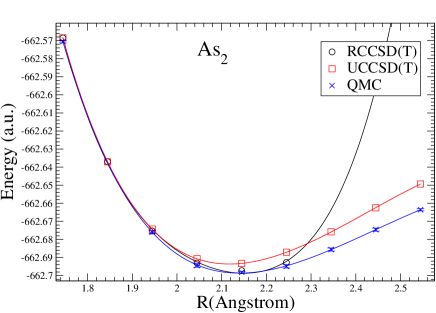
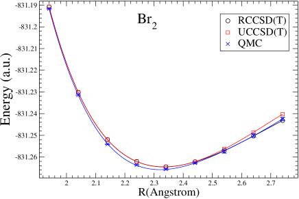
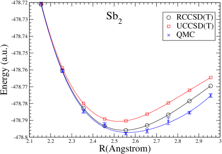
Figure 1: Potential energy curves of As₂, Br₂, and Sb₂ dimers (top to bottom panels, respectively) as obtained using RCCSD(T), UCCSD(T), and the present QMC methods. Calculations are done using cc-pVDZ-PP basis set. The solid lines are based on a polynomial fit to the results.

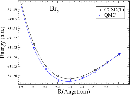
Figure 2: Potential energy surface of Br₂ within the cc-pVTZ-PP basis set, as calculated in RCCSD(T) and QMC. The solid lines are based on a polynomial fit to the results.

IV Results and discussion: dimers

We chose As₂, Br₂, and Sb₂ to study, as representatives of the first- and second-row post-d dimers. In Table 5, we summarize our study of their dissociation energy, equilibrium bondlength, and angular frequency of vibration using different methods, with the cc-pVDZ-PP and cc-pVTZ-PP basis sets. Spin-orbit effects in the experimental values ion_ref ; sontag are approximately removed exp_EA_moore .

Within each method, the equilibrium bondlength and angular frequency of vibrations are calculated from a fit to the potential energy curves of the dimers. The total energies for 8-9 geometries over the range $-0.4\leq R-R_{e}\leq 0.7$ Angstroms are fitted by 4-7th order polynomials, which gave consistent results. The dissociation energy of the dimers at the RHF, GGA, and B3LYP level of theories are calculated using the equilibrium bondlength at the same level of theory and using the same basis. For the correlated calculations, Table 5 tabulates the calculated equilibrium bondlength, but the dissociation energies that are shown were calculated using the equilibrium geometry optimized with CCSD(T)^∗, i.e., at the CCSD(T) level of theory with only the $ns$ and $np$ electrons correlated. This was done to facilitate the comparisons between the different methods. The dissociation energies at the respective optimized geometries will change by $1$ kcal/mol or less.

First, we discuss the density functional results. We have verified that the density functional GGA and hybrid B3LYP dissociation energies are already converged at the cc-pVTZ-PP basis set. Our dissociation energy results using cc-pVQZ-PP basis sets (not shown) differ from those reported at cc-pVTZ-PP by less than $1$ kcal/mol, the equilibrium bondlengths by less than $0.005$ Angstrom, and the angular frequencies by less than $1$ cm^-1. The density functional dissociation energies are in reasonable agreement with the experimental values. GGA overestimates the binding energies by $\approx 4-5$ kcal/mol, while B3LYP is in good agreement with experiment. The bondlengths are overestimated with GGA and slightly underestimated with B3LYP. Angular frequencies in GGA and B3LYP are in better agreement with each other, with the GGA frequencies being in good agreement with experimental values.

We next comment on the coupled cluster results with and without the frozen-core approximation. Contrary to the atomic properties, the dissociation energy, equilibrium bondlengths, and the angular frequency are more sensitive to the frozen-core approximation. The basis sets used in this study are optimized to recover the correlation energy of the valence electrons, and thus are less effective in accessing the core-valence correlation effects. In Refs. peterson1 ; peterson2 , the frozen-core CCSD(T) calculations of the spectroscopic properties of several dimers are in good agreement with the experimental values with the cc-PV5Z-PP basis sets.

We now focus on the QMC results, and their comparison with CCSD(T) and experiment. As mentioned, all of the QMC calculations were obtained using the UHF solution as trial wave function. QMC and CCSD(T) dissociation energies are in good agreement with each other. The QMC total energies for the atoms are within $1$ mE_h of the CCSD(T) values, as reported before in the study of the ionization energies in Sec. III.2. The QMC energies of the dimers, on the other hand, are below the CCSD(T) values by $\approx 1-3$ mE_h for the two basis sets and for all the studied dimers. This does not necessarily mean that QMC values are in better agreement with exact values, because these QMC calculations are non-variational (as is CCSD(T)). In our previous study of the first-row atoms and molecules where some exact values were available, our comparisons showed that the exact values often fell between the CCSD(T) and QMC values.gafqmc

The bondlengths and the angular frequency of vibrations obtained with QMC and CCSD(T) are in less good agreement with each other, compared to the dissociation energies. In Fig. 1, we show the potential energy curves of As₂, Br₂, and Sb₂ dimers within the cc-pVDZ-PP basis set, as calculated with QMC, and both RCCSD(T) and UCCSD(T) which are based on RHF and UHF reference states, respectively. In As₂/cc-pVDZ-PP, we could not obtain the RCCSD(T) energies for some of the geometries ($R\approx 2.25-2.45$ Angstroms) due to the lack of convergence, as can be seen in Fig. 1.

Figure 2 shows the potential energy surface of Br₂ within the cc-pVTZ-PP basis sets, as calculated using CCSD(T) and the present QMC. In this case, we show only the RCCSD(T) values, because we could not obtain a UHF solution in this system for the cc-pVTZ-PP basis set at the bondlengths shown.

For singlets, the RCCSD(T) is generally more accurate near the equilibrium bondlength, while UCCSD(T) performs better for larger bondlengths near the dissociation limit. Both the QMC and RCCSD(T) energies are in excellent agreement near the equilibrium bondlength (with QMC slightly lower). However, as the bondlength is stretched, RCCSD(T) becomes less accurate, and for relatively small bondlength stretching UCCSD(T) is also inaccurate H2O_Olsen ; garnet_N2 . QMC, on the other hand, has been shown to give a more uniform description across the whole potential energy surface in first-row molecules gafqmc ; gafqmc2 . Given these results, especially our benchmark study on N₂ gafqmc2 , it seems reasonable to speculate that a significant portion of the discrepancy at larger bondlengths between QMC and CCSD(T) is due to errors in the latter. Further study is needed to better establish this.

V Summary

To further benchmark the recently introduced phaseless auxiliary-field QMC method, we have applied it to heavier systems using a Gaussian basis. We performed a systematic study of the first- and second-row non-transition metal post-d elements using the consistent correlation basis sets cc-pVnZ-PP peterson1 ; peterson2 which employ a small-core relativistic pseudopotentials. Our results for the electron affinities and the first ionization potentials of these elements are in excellent agreement with similar results calculated using CCSD(T) over double-, triple-, and quadruple-zeta basis sets. The corresponding energies of the atoms and the ions agree with the CCSD(T) values, with an average difference of less than $1$ mE_h. Our results obtained using the quadruple zeta basis set are in excellent agreement with experimental results.

We also studied the dimers As₂, Br₂, and Sb₂ using cc-pVDZ-PP and cc-pVTZ-PP basis sets. At the triple-zeta level, the calculated spectroscopic properties are in good agreement with experiment. Our results for the dissociation energies are in excellent agreement with CCSD(T) within each basis set. The equilibrium bondlength and the angular frequency of vibrations are also in good agreement with similar CCSD(T) results considering the somewhat large statistical errors on the QMC results. The potential energy curves for all of these molecules are in good agreement with CCSD(T) for bondlengths smaller than the equilibrium bondlength. For larger bondlengths, and especially in As₂ and Sb₂, the QMC results deviate significantly ($\approx 10$ mE_h) from both RCCSD(T) and UCCSD(T). Both coupled cluster methods are less accurate in these regions H2O_Olsen ; garnet_N2 ; Musial_bartlett_F2 , and QMC has been shown to give better accuracy and a more uniform behavior in H₂O, N₂, and F₂ gafqmc ; gafqmc2 . The deviations between QMC and CCSD(T) here seem consistent with these benchmark results in lighter systems.

VI Acknowledgments:

This work is supported by ONR (N000149710049 and N000140510055), NSF (DMR-0535529), and ARO (48752PH) grants, and by the DOE computational materials science network (CMSN). Computations were carried out at the Center for Piezoelectrics by Design, the SciClone Cluster at the College of William and Mary, NCSA at UIUC, and SDSC at UCSD.

References

- (1) S. Zhang and H. Krakauer, Phys. Rev. Lett. 90, 136401 (2003).
- (2) W. A. Al-Saidi, S. Zhang, and H. Krakauer, J. Chem. Phys. 124, 224101(2006).
- (3) W. A. Al-Saidi, S. Zhang, and H. Krakauer (unpublished).
- (4) K. A. Peterson, J. Chem. Phys. 119, 11099 (2003).
- (5) K. A. Peterson, D. Figgen, E. Goll, H. Stoll, and M. Dolg, J. Chem. Phys. 119, 11113 (2003).
- (6) These basis sets can be obtained from the Extensible Computational Chemistry Environment Basis Set Database (http://www.emsl.pnl.gov/forms/basisform.html).
- (7) T. H. Dunning, Jr., J. Chem. Phys. 90, 1007 (1989).
- (8) D. E. Woon and T. H. Dunning, Jr, J. Chem. Phys. 98, 1358 (1993).
- (9) M. Dolg, J. Chem. Phys. 104, 4061 (1996).
- (10) W. Kohn, Rev. Mod. Phys. 71, 1253 (1999).
- (11) J. Olsen, P. Jorgensen, H. Koch, A. Balkova, and R. J. Bartlett, J. Chem. Phys. 104, 8007 (1995).
- (12) Garnet Kin-Lic Chan, Nihaly Kallay, and Jürgen Gauss, J. Chem. Phys. 121, 6110 (2004).
- (13) M. Musial and R. J. Bartlett, J. Chem. Phys. 122, 224102 (2005).
- (14) J. B. Anderson, J. Chem. Phys. 63, 1499 (1975).
- (15) W. M. C. Foulkes, L. Mitas, R. J. Needs, and G. Rajagopal, Rev. Mod. Phys. 71, 33 (2001).
- (16) S. Zhang, in Quantum Monte Carlo Methods in Physics and Chemistry, ed. by M. P. Nightingale and C. J. Umrigar, NATO ASI Series (Kluwer Academic Publishers, 1998). (cond-mat/9909090)
- (17) S. Zhang, H. Krakauer, W. Al-Saidi, and M. Suewattana, Comp. Phys. Comm. 169, 394 (2005).
- (18) Malliga Suewattana, W. Purwanto, S. Zhang, H. Krakauer, and E. J. Walter (unpublished).
- (19) W. A. Al-Saidi, H. Krakauer, and S. Zhang, Phys. Rev. B 73, 075103 (2006).
- (20) Naomi Rom, D. M. Charutz, and Daniel Neuhauser, Chem. Phys. Lett. 270, 382 (1997); R. Baer, M. Head-Gordon, and D. Neuhauser, J. Chem. Phys. 109, 6219 (1998).
- (21) P. L. Silvestrelli, S. Baroni, and R. Car, Phys. Rev. Lett. 71, 1148 (1993).
- (22) R. Blankenbecler, D. J. Scalapino, and R. L. Sugar, Phys. Rev. D 24, 2278 (1981).
- (23) G. Sugiyama and S. E. Koonin, Ann. Phys. (NY) 168, 1 (1986).
- (24) R. L. Stratonovich, Sov. Phys. Dokl. 2, 416 (1958); J. Hubbard, Phys. Rev. Lett. 3, 77 (1959).
- (25) S. Zhang, J. Carlson, and J. E. Gubernatis, Phys. Rev. B 55, 7464 (1997).
- (26) H. Hotop and W. C. Lineberger, J. Phys. Chem. Ref. Data. 14, 731 (1985).
- (27) C. E. Moore, Atomic Energy Levels, NSRDS-NBS 35, Office of Standard Reference Data (National Bureau of Standards, Washington, D.C., 1971).
- (28) T. P. Straatsma, E. Aprá, T. L. Windus, E. J. Bylaska, et. al., “NWChem, A Computational Chemistry Package for Parallel Computers, Version 4.6” (2004), Pacific Northwest National Laboratory, Richland, Washington 99352-0999, USA.
- (29) M. J. Frisch, G. W. Trucks, H. B. Schlegel, et. al., GAUSSIAN 98, Revision A.7, Gaussian Inc., Pittsburgh, PA, 1998.
- (30) K. P. Huber and G. Herzberg, Molecular Spectra and Molecular Structures. IV. Constants of Diatomic Molecules, Van Nostrand, New York, 1979.
- (31) J. P. Perdew, K. Burke, and M. Ernzerhof, Phys. Rev. Lett 77, 3865 (1996).
- (32) A. D. Becke, J. Chem. Phys. 98, 5648 (1993); C. Lee, W. Yang, and R. G. Parr, Phys. Rev. B 37, 785 (1992).
- (33) H. Sontag and R. Wever, J. Mol. Spectrosc. 91, 72 (1982).
- (34) S. Yockel, B. Mintz, and A. K. Wilson, J. Chem. Phys. 121, 60 (2004).
- (35) L. A. Curtiss, M. P. McGrath, Jean-Philippe Blaudeau, Nancy E. Davis, and Leo Radom, J. Chem. Phys. 103, 6104 (1995).