On the exact number of possibilities for cutting and reconnecting the tour of a traveling salesman with Lin-$k$-Opts

Abstract

When trying to find approximate solutions for the Traveling Salesman Problem with heuristic optimization algorithms, small moves called Lin-$k$-Opts are often used. In our paper, we provide exact formulas for the numbers of possible tours into which a randomly chosen tour can be changed with a Lin-$k$-Opt.

I Introduction: The Traveling Salesman Problem

Due to the simplicity of its formulation and the complexity of its exact solution, the traveling salesman problem (TSP) has been studied for a very long time geschichte and has drawn great attention from various fields, such as applied mathematics, computational physics, and operations research. The traveling salesman faces the problem to find the shortest closed tour through a given set of nodes, touching each of the $N$ nodes exactly once and returning to the starting node at the end geschichte ; Lawler . Hereby the salesman knows the distances $d(i,j)$ between all pairs $(i,j)$ of nodes, which are usually given as some constant non-negative values, either in units of length or of time. The costs ${\cal H}$ of a configuration $\sigma$ are therefore given as the sum of the distances of the used edges. If denoting a configuration as a permutation $\sigma$ of the numbers $\{1,\dots,N\}$, the costs can be written as

$${\cal H}(\sigma)=d(\sigma(N),\sigma(1))+\sum_{i=1}^{N-1}d(\sigma(i),\sigma(i+1)).$$ (1)

A TSP instance is called symmetric if $d(i,j)=d(j,i)$ for all pairs $(i,j)$ of nodes. For a symmetric TSP, the costs for going through the tour in a clockwise direction are the same as going through in an anticlockwise direction. Thus, these two tours are to be considered as identical.

As the time for determining the optimum solution of a proposed TSP instance grows exponentially with the system size, the number $N$ of nodes, a large variety of heuristics has been developed in order to solve this problem approximately. Besides the application of several different construction heuristics Reinelt , which were either specifically designed for the TSP or altered in order to enable their application to the TSP, the TSP has been tackled with various general-purpose improvement heuristics, like Simulated Annealing Kirk and related algorithms such as Threshold Accepting TA ; Pablo , the Great Deluge Algorithm GDA ; Sintflut ; Dueckbuch , algorithms based on the Tsallis statistics Penna , Simulated and Parallel Tempering (methods described in MarinariParisi ; ParallelTempering2 ; ParallelTempering1 ; ParallelTempering1a ; ParallelTempering1b ), and Search Space Smoothing JunGu ; SSS ; SSSKonkurrenz . Furthermore Genetic Algorithms Schoeneburg ; Goldbergkommune ; Holland , Tabu Search Tabu1 and Scatter Search Tabu1 ; Tabu2 , and even Ant Colony Optimization aco , Particle Swarm Optimization psofull ; pso ; psobook , and other biologically motivated algorithms Antlion have been applied to the TSP. The quality of these algorithms is compared by creating solutions for benchmark instances, one of which is shown in Fig. 1.

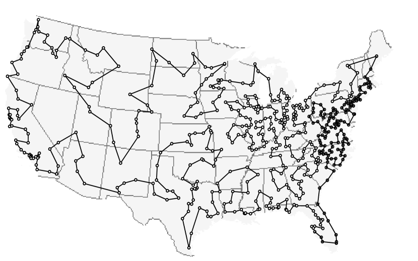
Figure 1: The optimum solution of the ATT532 benchmark TSP instance containing the 532 AT&T switch locations in the United States of America: this benchmark instance is part of Reinelt’s benchmark library TSPLIB95 TSPLIB95 . The optimum solution was created with the Searching for Backbones algorithm sfb ; sfb2 , making use of the Lin-2-Opt and the Lin-3-Opt, which are shown in Figs. 3 and 4.

Most of these improvement heuristics apply a series of so-called small moves to a current configuration or a set of configurations. In this context, the move being small means that it does not change a configuration very much, such that usually the cost of the new tentative configuration which is to be accepted or rejected according to the acceptance criterion of the improvement heuristics does not differ very much from the cost of the current configuration. This method of using only small moves is called the Local Search approach, as the small moves lead to tentative new configurations, which are close to the previous configuration according to some metric like the Hamming distance for the TSP: the Hamming distance between two tours is given by the number of different edges.

II The Smallest Moves

II.1 The Exchange

Figure 2: The Exchange (left) and the Node Insertion Move (right)

One move which does not change a configuration very much is the Exchange (EXC), which is sometimes also called Swap and which is shown in Fig. 2. The Exchange exchanges two randomly selected nodes in the tour. Thus, from a proposed configuration, $N\times(N-1)/2$ other configurations can be reached, such that the neighborhood of a configuration generated by this move has a size of order ${\cal O}(N^{2})$.

II.2 The Node Insertion Move

Another small move is the Node Insertion Move (NIM), which is also called Jump. It is also shown in Fig. 2. The Node Insertion Move randomly selects a node and an edge. It removes the randomly chosen node from its original position and places it between the end points of the randomly selected edge, which is cut for this purpose. The neighborhood size generated by this move is $N\times(N-2)$ and thus also of order ${\cal O}(N^{2})$.

II.3 The Lin-2-Opt

Figure 3: The Lin-2-Opt

Lin introduced a further small move, which is called Lin-2-Opt (L2O) Lin ; LinK : as shown in Fig. 3, it cuts two edges of the tour, turns the direction of one of the two partial sequences around, and reconnects these two sequences in a new way. For symmetric TSP instances, only the two removed edges and the two added edges have to be considered when calculating the cost difference created by this move. For these symmetric TSPs, it plays no role which of the two partial sequences is turned around when performing the move, due to the identical cost function value for moving through clockwisely or anticlockwisely. In the symmetric case, on which we will concentrate throughout this paper, the move creates a neighborhood of size $N\times(N-3)/2$ and thus of order ${\cal O}(N^{2})$. Please note that a move cutting two edges after neighboring nodes does not lead to a new configuration, such that the neighborhood size is not $N\times(N-1)/2$, a false value which is sometimes found in the literature.

The Lin-2-Opt turned out to provide better results for the symmetric Traveling Salesman Problem than the Exchange. The reason for this quality difference was explained analytically by Stadler and Schnabl. In their paper Stadler , they basically found out that the results are the better the less edges are cut: the Lin-2-Opt cuts only two edges whereas the Exchange cuts four. But they also reported results that the Lin-3-Opt cutting three edges leads to an even better quality of the solutions than the Lin-2-Opt, what contradicted their results at first sight, but they explained this finding with the larger neighborhood size of the Lin-3-Opt.

III The Lin-3-Opt

Figure 4: The four possibilities how to change a tour with a Lin-3-Opt

The next larger move to the Lin-2-Opt is the Lin-3-Opt (L3O): the Lin-3-Opt removes three edges of the tour and reconnects the three partial sequences to some new closed tour. In contrast to the smallest moves for which there is only one possibility to create a new tour, there are four possibilities in the case of the symmetric TSP how to create a new tour with three new edges with the Lin-3-Opt if each of the partial sequences contains at least two nodes. These four possibilities are shown in Fig. 4. Please note that we count only the number of “true” possibilities here, i.e., only those cases in which the tour contains three edges which were not part formerly in the tour, as otherwise the move would e.g. only be a Lin-2-Opt. If one of the partial sequences contains only one node and the other two at least two nodes each, then only one possibility for a “true” Lin-3-Opt remains. If even two of the three partial sequences do only contain one node, then there is no possibility left to reconnect the three sequences without reusing at least one of the edges which was cut. Analogously, there is one possibility for the Lin-2-Opt, if both partial sequences contain at least two nodes each, otherwise there is no possibility.

If looking closely at the four variants of the Lin-3-Opt in Fig. 4, one finds that the resulting configurations could also be generated by a sequence of Lin-2-Opts: for the upper left variant in Fig. 4, three Lin-2-Opts would be needed, whereas only two Lin-2-Opts would be sufficient for the other three variants. Thus, one might ask whether the Lin-3-Opt is necessary as a move as a few Lin-2-Opts could do the same job. However, due to the acceptance criteria of the improvement heuristics, it might be that at least one of the Lin-2-Opts would be rejected whereas the combined Lin-3-Opt move could be accepted. Thus, it is often advantageous also to implement these next-higher-order moves in order to overcome the barriers in the energy landscape of the small moves.

Now the question arises how large the neighborhood size of a Lin-3-Opt is. Of course, it has to be of order ${\cal O}(N^{3})$, as three edges to be removed are randomly selected out of $N$ edges. However, for the calculation of the exact number of possibilities one has to distinguish between the case in which all partial sequences contain at least two nodes each and the case in which exactly one partial sequence contains only one node.

Please note that the Node Insertion Move, which was introduced earlier, is the special case of the Lin-3-Opt in which one of the partial sequences only contains one node. But in the special case that one of the two next nearest edges to the randomly chosen node is selected, the NIM corresponds to a Lin-2-Opt. As the number of cut edges of the NIM is 3, such that this move is basically a Lin-3-Opt, but as the neighborhood size of this move is of order ${\cal O}(N^{2})$, this move is also sometimes called Lin-2.5-Opt.

IV Higher-order Moves

One can go on to even higher-order Lin-$k$-Opts: the Lin-4-Opt cuts four edges of the tour and reconnects the four created partial sequences in a new way. If every partial sequence contains at least two nodes, there are 25 possibilities for a true Lin-4-Opt to reconnect the partial sequences to a closed feasible tour. The neighborhood size of this move is of order ${\cal O}(N^{4})$.

The Exchange, which was also introduced earlier, is usually a special case of a Lin-4-Opt. Only if the two nodes which are to be exchanged are direct neighbors of each other or if there is exactly one node between them, then the move is equivalent to a Lin-2-Opt.

One can increase the number $k$ of deleted edges further and further. However, by doing so, one gradually loses the advantage of the Local Search approach, in which, due to the similarity of the configurations, their cost values do not differ much. In the extreme, the Lin-$N$-Opt would lead to a randomly chosen new configuration, the cost value of which is not related to the cost value of the previous configuration at all. Moving away from the Local Search approach, the probability for getting an acceptable new configuration among the many more neighboring configurations with cost values in a much larger interval strongly decreases due to the finite available computing time. When using the Local Search approach, it turns out that using the smallest possible move only is only optimal in the case of very short computing times. With increasing computing time, a well chosen combination of the smallest moves and their next larger variants becomes optimal. Here the optimization run has more time to search through a larger neighborhood. The next larger moves enable the system to overcome barriers in the energy landscape formed by the small moves only. Of course, one can extend this approach and also include moves with the next larger $k$ and spend even more computing time.

However, for some difficult optimization problems, an approach based on small moves and their next larger variants is not sufficient Schrimpf . There indeed large moves have to be used. A successful approach here are the Ruin & Recreate moves, which destroy a configuration to some extent and rebuild it according to a given rule set. They work in a different way than the small moves, which completely randomly select a way to change the configuration. In contrast, the Ruin & Recreate moves contain constructive elements in order to result in good configurations. Also for problems like the TSP, for which small moves basically work, well designed Ruin & Recreate moves are superior to the small moves Schrimpf . However, the development of excellent Ruin & Recreate moves is rather difficult, it is indeed an optimization problem itself, whereas the application of the Local Search approach, which simply intends to “change the configuration a little bit”, is rather straightforward and also usually quite successful in producing good solutions, such that it is mostly used.

Sometimes one needs to know the exact size of the neighborhood generated by the implemented moves for relating it to the available computing time or for tuning an optimization algorithm like Tabu Search. Naturally, one is aware of the neighborhood size of a Lin-$k$-Opt being of order ${\cal O}(N^{k})$. The aim of this paper is to provide exact numbers for the neighborhood size. For deriving the neighborhood size of the Lin-3-Opt and of even larger Lin-$k$-Opts, we will start with the determination of the number of possibilities for reconnecting partial sequences to a complete tour with a true Lin-$k$-Opt in Sec. V. There we will find laws how many possibilities exist depending on the number of partial sequences containing only one node and their spatial neighborhood relation to each other. Having this distinction at hand, we will calculate the corresponding numbers of possibilities for cutting the tour in Sec. VI.

V Number of possibilities for reconnecting the tour with a Lin-$k$-Opt

V.1 Special case

V.1.1 Number of overall possibilities

For the calculation of the number of possibilities for reconnecting the tour, we want to start out with the special case that each partial sequence contains at least two nodes. A Lin-$k$-Opt cuts the tour into $k$ partial sequences. The overall number of possibilities to reconnect them to a closed tour containing all nodes can be obtained when imagining the following scenario: one randomly selects one of the partial sequences and fixes its direction. (This has to be done for the symmetric TSP for which a tour and its mirror tour are degenerate) This first partial sequence serves as a starting sequence for the new tour to be constructed. Then one randomly selects one out of the $k-1$ remaining partial sequences and adds it to the already existing partial tour. There are two possible ways of adding it, one for each direction of the partial sequence. Thus, one gets a new system with only $k-1$ partial sequences. The number of possibilities to construct a new feasible tour is thus given as

$$P(k)=2(k-1)P(k-1).$$ (2)

This recursive formula can be easily desolved to

$$P(k)=2^{k-1}(k-1)!.$$ (3)

V.1.2 Number of true Lin-$k$-Opts

However, this overall set of possibilities contains many variants in which old edges which were cut are reused in the new configuration, such that the move is not a true Lin-$k$-Opt. Thus, in order to get the number of true Lin-$k$-Opts, those variants have to be subtracted from the overall number. As there are ${k\choose i}$ possibilities to choose $i$ old edges for the new tour if there were overall $k$ deleted edges, the number of true Lin-$k$-Opts is given by the recursive formula

$$T(k)=2^{k-1}(k-1)!-\sum_{i=0}^{k-1}{k\choose i}T(i)\,\mbox{with}\,T(0)=1.$$ (4)

The starting point of this recursion is $T(0)=1$, as there is one possibility for the Lin-0-Opt, the identity move, in which no edge is changed. Table 1 gives an overview of the numbers of true Lin-$k$-Opts for small $k$, in the case that each partial sequence contains at least two nodes and that the TSP is symmetric. We find that there is one Lin-0-Opt, the identity move, no Lin-1-Opt, as by cutting only one edge no new tour can be formed, one Lin-2-Opt, four Lin-3-Opts, and so on. In the case of an asymmetric TSP, each number here has to be multiplied by a factor of 2.

Table 1: Number of true Lin-$k$-Opts if the TSP is symmetric and if every partial sequence contains at least 2 nodes

$k$	$T(k)$
0	1
1	0
2	1
3	4
4	25
5	208
6	2121

V.2 General case

V.2.1 Number of overall possibilities

In the general case, not every partial sequence contains at least two nodes. There might be sequences containing only one node which are surrounded by two sequences containing more than one node in the old tour. Furthermore, there might be tuples of neighboring sequences containing only one node each which are surrounded by two sequences containing more than one node, and so on.

Let $\alpha_{0}$ be the number of the partial sequences containing more than one node, $\alpha_{1}$ be the number of sequences containing only one node and surrounded by two sequences containing more than one node in the old tour, $\alpha_{2}$ be the number of tuples of one-node-sequences surrounded by two sequences containing more than one node in the old tour, $\alpha_{3}$ be the number of triples of one-node-sequences surrounded by two sequences containing more than one node in the old tour, and so on. We will see that $P$ and $T$ are no longer functions of $k$ only, but depend on the entries of the vector $\vec{\alpha}=(\alpha_{0},\alpha_{1},\dots)$.

In the following, the assumption shall hold that not every edge of the tour is cut, such that $k<N$ and $\alpha_{0}>0$. Thus, one can always choose a partial sequence consisting of two or more nodes as a starting point for the creation of a new tour and fix its direction, as we only consider the symmetric TSP here.

Starting with this fixed partial sequence, a new feasible tour containing all nodes can be constructed by iteratively selecting an other partial sequence and adding it to the end of the growing partial tour. For the overall number of possibilities for construcing a new tour, it plays no role whether one-node-sequences were side by side in the old tour or not. Thus, the number of possibilities $P(\vec{\alpha})$ is simply given as

$$P(\vec{\alpha})=P(\alpha_{0},k-\alpha_{0},0,\dots,0).$$ (5)

There are two possible ways for adding a partial sequence containing at least two nodes, but only one possibility for adding a sequence with only one node. Thus, analogously to the result above we get the result

$$P(\vec{\alpha})=2^{\alpha_{0}-1}(k-1)!.$$ (6)

For the asymmetric TSP, this number has to be multiplied with 2.

V.2.2 Number of true Lin-$k$-Opts

When calculating the number of true Lin-$k$-Opts, we need to consider the spatial arrangement of the one-node-sequences in the old tour. We have to distinguish between single one-node-sequences, tuples, triples, quadruples, and so on, i.e., we have to consider the $i$-tuples for each $i$ separately. Contrarily, we have no problems with the spatial arrangement of partial sequences with at least two nodes. In order to get the number of true Lin-$k$-Opts, we want to use a trick by artificially blowing up partial sequences with only one node to sequences with two nodes. Let us first consider here that there are not only partial sequences with at least two nodes but also isolated partial sequences with only one node. (We thus first leave out the tuples, triples, …of single-node-sequences in our considerations, but it does not matter here whether there are any such structures.) We extend one one-node sequence to two nodes by doubling the node. Thus, one gets $T(\alpha_{0}+1,\alpha_{1}-1,\dots)$ possibilities for performing a true Lin-$k$-Opt instead of $T(\alpha_{0},\alpha_{1},\dots)$ possibilities. By changing the direction of this blown-up sequence, one can connect it – in contrast to before as it consisted of only one node – to those nodes of the neighboring parts to which it was connected before. There are two possibilities to connect it this way to one of the two neighboring partial sequences and one possibility to connect it this way to both of them. But these cases are forbidden, such that we have to subtract the number of these possibilities in which they get connected and we achieve the recursive formula

$$\begin{array}[]{lll}\displaystyle T(\vec{\alpha})=\frac{1}{2}(&&T(\alpha_{0}+1,\alpha_{1}-1,\alpha_{2},\dots)\cr\displaystyle&-2&T(\alpha_{0},\alpha_{1}-1,\alpha_{2},\dots)\cr\displaystyle&-&T(\alpha_{0}-1,\alpha_{1}-1,\alpha_{2},\dots).\cr\end{array}$$ (7)

Please note that the resulting number has to be divided by 2, as a partial sequence with only one node cannot be inserted in two different directions.

Analogously, one can derive a formula if there are tuples of neighboring sequences with only one node each. Here one expands one of the two partial sequences to two nodes, such that there is one tuple less, but one isolated one-node-sequence more and one longer sequence more. Analogously to above, the false possibilities must be subtracted and the result divided by 2, such that we get the formula

$$\begin{array}[]{lll}\displaystyle T(\vec{\alpha})=\frac{1}{2}(&&T(\alpha_{0}+1,\alpha_{1}+1,\alpha_{2}-1,\alpha_{3},\dots)\cr\displaystyle&-&T(\alpha_{0},\alpha_{1}+1,\alpha_{2}-1,\alpha_{3},\dots)\cr\displaystyle&-&T(\alpha_{0}+1,\alpha_{1},\alpha_{2}-1,\alpha_{3},\dots)\cr\displaystyle&-&T(\alpha_{0},\alpha_{1},\alpha_{2}-1,\alpha_{3},\dots)).\cr\end{array}$$ (8)

For all longer groups of single-node-sequences, like triples and quadruples, there is one common approach. Here it is appropriate to blow up a single-node-sequence at the frontier, such that the following recursive formula is achieved:

$$\begin{array}[]{llll}\displaystyle T(\vec{\alpha})=\displaystyle\frac{1}{2}(&&T(&\alpha_{0}+1,\alpha_{1},\dots,\alpha_{i-1}+1,\alpha_{i}-1,\cr&&&\alpha_{i+1},\dots)\cr\displaystyle&-&T(&\alpha_{0},\alpha_{1},\dots,\alpha_{i-1}+1,\alpha_{i}-1,\cr&&&\alpha_{i+1},\dots)\cr\displaystyle&-&T(&\alpha_{0}+1,\alpha_{1},\dots,\alpha_{i-2}+1,\alpha_{i-1},\alpha_{i}-1,\cr&&&\alpha_{i+1},\dots)\cr\displaystyle&-&T(&\alpha_{0},\alpha_{1},\dots,\alpha_{i-2}+1,\alpha_{i-1},\alpha_{i}-1,\cr&&&\alpha_{i+1},\dots))\cr\end{array}$$ (9)

Generally, one should proceed with the recursion in the following way: first, those non-zero $\alpha_{i}$ should vanish for which $i$ is maximal. This approach should be iterated with decreasing $i$ until one ends up for a formula for tours with partial sequences consisting of at least two nodes each for which we can use the formula for the special case.

VI Number of possibilities for cutting the tour with a Lin-$k$-Opt

VI.1 Special Case

Table 2: Number of possibilities for cutting the tour of a traveling salesman if each partial sequence shall contain at least two nodes: $k$ denotes the number of cuts of the Lin-$k$-Opt, $C(k)$ the number of possibilities.

$k$	$C(k)$
2	$N\times(N-3)/2$
3	$N\times(N-4)(N-5)/3!$
4	$N\times(N-5)(N-6)(N-7)/4!$
5	$N\times(N-6)(N-7)(N-8)(N-9)/5!$

After having determined the number of possibilities to reconnect partial sequences to a closed tour with a true Lin-$k$-Opt, we still have to determine the number of possibilities for cutting the tour in order to create these partial sequences. We again start out with the special case in which every partial sequence to be created shall contain at least two nodes. By empirical going through all possibilities, we found the formulas which are given in Tab. 2. From this result, we deduce a general formula for the possibilities $C(k)$ for the Lin-$k$-Opt:

$$C(k)=N\times\prod_{i=1}^{k-1}(N-k-i)\times\frac{\displaystyle 1}{\displaystyle k!}=\frac{\displaystyle N}{\displaystyle N-k}\times{N-k\choose k}$$ (10)

Thus, we find here that the neighborhood created by a Lin-$k$-Opt is of order ${\cal O}(N^{k})$.

VI.2 General Case

Table 3: Number of possibilities for cutting the tour of a traveling salesman: $k$ denotes the overall number of cuts performed by the Lin-$k$-Opt, $\beta_{1}$, $\beta_{2}$, $\beta_{3}$, and $\beta_{4}$ denote the number of $1$-, $2$-, $3$-, and $4$-type multicuts as defined in the text. Only $\beta_{i}$-values for $i\leq 4$ are considered here in our examples. For the Lin-6-Opt, only some special cases are considered. The number $C$ of possibilities depends on all these numbers. All these formulas for $C(\vec{\beta})$ were found by hand.

$k$	$\beta_{1}$	$\beta_{2}$	$\beta_{3}$	$\beta_{4}$	$C$
2	2	0	0	0	$N\times(N-3)/2$
	0	1	0	0	$N$
3	3	0	0	0	$N\times(N-4)(N-5)/3!$
	1	1	0	0	$N\times(N-4)$
	0	0	1	0	$N$
4	4	0	0	0	$N\times(N-5)(N-6)(N-7)/4!$
	2	1	0	0	$N\times(N-5)(N-6)/2$
	0	2	0	0	$N\times(N-5)/2$
	1	0	1	0	$N\times(N-5)$
	0	0	0	1	$N$
5	5	0	0	0	$N\times(N-6)(N-7)(N-8)(N-9)/5!$
	3	1	0	0	$N\times(N-6)(N-7)(N-8)/3!$
	1	2	0	0	$N\times(N-6)(N-7)/2$
	2	0	1	0	$N\times(N-6)(N-7)/2$
	0	1	1	0	$N\times(N-6)$
	1	0	0	1	$N\times(N-6)$
6	2	2	0	0	$N\times(N-7)(N-8)(N-9)/2/2$
	0	3	0	0	$N\times(N-7)(N-8)/3!$
	3	0	1	0	$N\times(N-7)(N-8)(N-9)/3!$
	1	1	1	0	$N\times(N-7)(N-8)$
	0	0	2	0	$N\times(N-7)/2$
	2	0	0	1	$N\times(N-7)(N-8)/2$
	0	1	0	1	$N\times(N-7)$

In the general case, an arbitrary Lin-$k$-Opt can also lead to partial sequences containing only one node. Here we have to distinguish between various types of cuts: The cuts introduced by a Lin-$k$-Opt can be isolated, i.e., they are between two sequences with more than one node each. Then they can lead to isolated nodes which are between two partial sequences with more than one node each, and so on. Let us view this from the point of view of the cuts of the tour. All in all, a Lin-$k$-Opt generally leads to $k$ cuts in the tour. Let us denote an $i$-type multicut (with $1\leq i\leq k$) at position $j$ (with $1\leq j\leq N$) as the scenario that the tour is cut at $i$ successive positions after the node with the tour position number $j$. Thus, the tour is cut by an $i$-type multicut successively between pairs of nodes with the tour position numbers $(j,j+1),(j+1,j+2),\dots,(j+i-1,j+i)$.

Furthermore, let $\beta_{i}$ be the number of $i$-type multicuts: $\beta_{1}$ is the number of isolated cuts. $\beta_{2}$ is the number of 2-type multicuts by which the tour is cut after two successive tour positions such that a partial sequence containing only one node is created, surrounded by two sequences containing more than one node. Thus, $\beta_{2}$ is also the number of isolated nodes surrounded by longer sequences and is thus identical with $\alpha_{1}$. Analogously, 3-type multicuts lead to tuples of nodes which are surrounded by partial sequences with more than one node, thus, $\beta_{3}$ is the number $\alpha_{2}$ of these tuples. Analogously, 4-type multicuts lead to triples of sequences containing only one node each, and so on. Generally, we have for all $i\geq 1$ that

$$\alpha_{i}=\beta_{i+1}$$ (11)

of the last section, but for $i=0$ the situation is different: each $i$-type multicut produces a further sequence consisting of at least two nodes, such that we have

$$\alpha_{0}=\sum_{i=1}^{k}\beta_{i}.$$ (12)

Please note that $\alpha_{0}$ is both the number of these longer partial sequences and the number of all $i$-type multicuts. The overall number $k$ of cuts can be expressed as

$$k=\sum_{i=1}^{k}i\beta_{i}.$$ (13)

In this general case, the number $C$ of ways of cutting the tour also depends not only on $k$, but on the entries of the vector $\vec{\beta}=(\beta_{1},\beta_{2},\dots,\beta_{k})$. As Tab. 3 shows, the order of the neighborhood size is now given as ${\cal O}(N^{\alpha_{0}})$. From these examples in the table, we empirically derive the formula

$$C(\vec{\beta})=N\times\prod_{i=1}^{\sum_{j=1}^{k}\beta_{j}-1}(N-k-i)\times\frac{\displaystyle 1}{\displaystyle\prod_{i=1}^{k}\beta_{i}!}$$ (14)

for the number of possibilities for cutting a tour with a Lin-$k$-Opt, leading to $\beta_{i}$ many $i$-type multicuts. Please note that if the upper index of a product is smaller than the lower index, then this so-called empty product is 1. This formula can be rewritten to

$$C(\vec{\beta})=\frac{\displaystyle N}{\displaystyle N-k}\times{N-k\choose\alpha_{0}}\times\frac{\displaystyle\alpha_{0}!}{\displaystyle\prod_{i=1}^{k}\beta_{i}!}$$ (15)

making use of $\alpha_{0}$ being the sum of all $\beta_{i}$. Please note that Eq. (10) for the special case with each sequence containing at least two nodes is a special case of Eq. (15).

The numbers for cutting a tour in partial sequences in this section were first found by hand for the examples given in Tabs. 2 and 3, then the general formulas were intuitively deduced from these. After that the correctness of these fomulas was checked by computer programs up to $k=20$ for the special case and for all variations of the general case.

VII Quality of the Results Achieved with Various Moves

Table 4: Results for the Greedy Algorithm using small moves (Exchange, Node Insertion Move, and Lin-2-Opt) and the variants of the Lin-3-Opt: for each instance, 100 optimization runs were performed, starting with a random configuration and performing a specific number (given in the text) of the corresponding move.

instance	move	minimum	maximum	mean value	$\pm$	error
BEER127	EXC	159705.087	208409.703	182672.403	$\pm$	977.4
	NIM	132898.075	161648.200	146418.726	$\pm$	596.4
	L2O	121178.315	138126.861	129964.407	$\pm$	325.5
	all small	119331.431	134236.701	126605.995	$\pm$	305.2
	L3O1	119218.371	131235.436	125118.494	$\pm$	254.3
	L3O2	120935.053	133226.981	125888.805	$\pm$	260.4
	L3O3	118589.344	127980.167	121981.992	$\pm$	187.4
	L3O4	118899.537	127588.470	121928.533	$\pm$	187.4
	L3Oall	118629.043	127881.507	121396.175	$\pm$	194.1
LIN318	EXC	90116.6104	127763.120	110660.750	$\pm$	628.5
	NIM	59992.7967	78436.1451	68407.9569	$\pm$	376.2
	L2O	45115.9243	49971.4471	47276.4710	$\pm$	95.0
	all small	43488.2914	47875.0510	45743.4573	$\pm$	78.9
	L3O1	43883.1117	46992.0997	45210.0271	$\pm$	63.9
	L3O2	44209.8503	47368.0175	45466.4980	$\pm$	66.1
	L3O3	42863.7951	44822.3800	43632.8142	$\pm$	39.5
	L3O4	42626.6703	45173.6630	43534.8133	$\pm$	44.4
	L3Oall	42401.9352	44514.0820	43518.6735	$\pm$	40.7
PCB442	EXC	112322.878	142974.558	129290.471	$\pm$	708.4
	NIM	64129.9159	79939.0300	70764.4069	$\pm$	296.7
	L2O	54682.4205	59026.1119	56614.6608	$\pm$	82.3
	all small	52589.4816	56840.8241	54660.7005	$\pm$	76.3
	L3O1	53547.9002	56348.0251	54850.7759	$\pm$	60.7
	L3O2	52975.6709	57838.1568	54847.6013	$\pm$	85.7
	L3O3	51658.9173	54163.2202	52689.2427	$\pm$	47.9
	L3O4	51627.2806	53519.6159	52545.4050	$\pm$	41.0
	L3Oall	51480.2480	53892.2666	52493.4278	$\pm$	44.5
ATT532	EXC	69294	91946	80037.86	$\pm$	449.7
	NIM	37691	47862	42460.43	$\pm$	212.1
	L2O	29960	32026	30867.73	$\pm$	42.2
	all small	29069	30530	29689.64	$\pm$	31.1
	L3O1	28716	30639	29732.22	$\pm$	33.7
	L3O2	29229	30817	30031.61	$\pm$	30.7
	L3O3	28275	29369	28692.05	$\pm$	22.8
	L3O4	28076	29159	28673.47	$\pm$	21.4
	L3Oall	28281	29102	28718.27	$\pm$	19.6
NRW1379	EXC	164670.848	196316.798	181017.337	$\pm$	607.0
	NIM	89353.7705	105344.742	94486.5234	$\pm$	294.3
	L2O	62862.6385	64887.1349	64046.8071	$\pm$	42.9
	all small	60334.7758	62208.5391	61154.0388	$\pm$	39.4
	L3O1	64624.4812	66712.2867	65611.2830	$\pm$	35.6
	L3O2	63267.3838	64788.3074	64008.2578	$\pm$	37.1
	L3O3	58730.9852	59768.7048	59199.8516	$\pm$	25.4
	L3O4	58727.9973	59656.5893	59173.3947	$\pm$	23.5
	L3Oall	58650.2000	60077.9761	59307.8550	$\pm$	26.1

Finally, we want to ask which quality of solutions can be achieved with the various moves. Here we concentrate on a comparison of the quality which can be achieved by the “power” of the moves only, thus, we do not use some elaborate underlying heuristics like those mentioned in the introduction, bnt use the simplest algorithm, which is often called Greedy Algorithm, here: starting out from a randomly created configuration $\sigma_{0}$, a series of moves is applied to the system. Each move chooses randomly a way how to change the current configuration $\sigma_{i}$ into a new configuration $\sigma_{i+1}$. A move is only accepted by the Greedy Algorithm if it does not lead to a deterioration, i.e., if the length ${\cal H}(\sigma_{i+1})$ of the tentative new tour is as long as or is shorter than the length ${\cal H}(\sigma_{i})$ of the current tour. After the acceptance of the move $\sigma_{i}\to\sigma_{i+1}$, the system tries to move from the configuration $\sigma_{i+1}$ to a new configuration. In case of rejection of the move $\sigma_{i}\to\sigma_{i+1}$, one sets $\sigma_{i+1}=\sigma_{i}$ and proceeds as above.

Table 4 shows the minimum, maximum, and average quality of solutions which can be achieved with the various moves for five different TSP benchmark instances which were taken from Reinelt’s TSPLIB95 TSPLIB95 and which vary in size between $N=127$ and $N=1379$. In order to be quite sure to end up in a local minimum, we used $50\times N^{2}$ move trials if using either the Exchange or the Node Insertion Move or the Lin-2-Opt. If comparing the results achieved with these small moves, we find that the Lin-2-Opt leads to the best results and the Exchange leads to the worst results, a result which is in accordance with the theoretical derivations in Stadler . Now one can also mix these moves in the way that a general move routine calls each of these three moves with equal probability. The next line in Tab. 4 shows that the results, which were taken after $150\times N^{2}$ move trials, are better for this mixture than for any of the three moves themselves. This is of course due to the larger neighborhood size of this mixture.

Then we provide the results for the four variants of the Lin-3-Opt, for which the results were taken after $10\times N^{3}$ move trials (A few test runs froze after $1-2\times N^{3}$ move trials), and for a mixture (Here we call each of the four variants with equal probability), for which the results were taken after $20\times N^{3}$ move trials. If we denote the tour position numbers after which the tour is cut by the Lin-3-Opt as $i$, $j$, and $k$ with $i<j<k$ and their successive tour position numbers as $i_{+}$, $j_{+}$, and $k_{+}$, we can write the cut tour as follows:

$$\begin{array}[]{cc|ccc|ccc|cc}\dots&\sigma(i)&\sigma(i_{+})&\dots&\sigma(j)&\sigma(j_{+})&\dots&\sigma(k)&\sigma(k_{+})&\dots\end{array}$$

Please note that the tour is of course closed, such that the partial sequence starting at $\sigma(k_{+})$ ends with $\sigma(i)$. If $j\neq i_{+}$, $k\neq j_{+}$, and $i\neq k_{+}$, there are four possibilities to reconnect the three partial sequences with a true Lin-3-Opt:

$$\begin{array}[]{ccc|ccc|ccc|cc}\mbox{L3O1:}&\dots&\sigma(i)&\sigma(j_{+})&\dots&\sigma(k)&\sigma(i_{+})&\dots&\sigma(j)&\sigma(k_{+})&\dots\cr\mbox{L3O2:}&\dots&\sigma(i)&\sigma(j)&\dots&\sigma(i_{+})&\sigma(k)&\dots&\sigma(j_{+})&\sigma(k_{+})&\dots\cr\mbox{L3O3:}&\dots&\sigma(i)&\sigma(j_{+})&\dots&\sigma(k)&\sigma(j)&\dots&\sigma(i_{+})&\sigma(k_{+})&\dots\cr\mbox{L3O4:}&\dots&\sigma(i)&\sigma(k)&\dots&\sigma(j_{+})&\sigma(i_{+})&\dots&\sigma(j)&\sigma(k_{+})&\dots\cr\end{array}$$

Table 4 shows that there are some differences in the qualities of the results achieved with the four variants of the Lin-3-Opt and that the mixture provides the best results for the three smaller instances, whereas two variants are on average better than the mixture for the instances with $N=532$ and $N=1379$. Comparing these results with the results for the small moves, we find that the four variants of the Lin-3-Opt lead to a much better quality of the results than the small moves, which is in accordance with the results in 3OptBesser . As Stadler and Schnabl already mentioned in Stadler , this better quality of the results has to be expected because of the much larger neighborhood size of the Lin-3-Opts.

Table 5: Results for the Greedy Algorithm using two types of Lin-4-Opts: for each instance, 100 optimization runs were performed, starting with a random configuration and performing $N^{4}$ times one variant of the Lin-4-Opt with the Greedy acceptance criterion. As the computing time is rather large, only small instances are considered.

instance	move	minimum	maximum	mean value	$\pm$	error
BEER127	L4O1	123767.073	134986.024	129588.275	$\pm$	244.2
	L4O2	121407.255	131300.030	125622.863	$\pm$	214.7
LIN318	L4O1	45184.3246	48569.5839	46740.9896	$\pm$	72.2
	L4O2	44539.2015	46932.1063	45451.7793	$\pm$	48.3
PCB442	L4O1	55673.1534	58855.2662	57381.3213	$\pm$	71.3
	L4O2	53793.3942	56843.4938	55209.2331	$\pm$	64.0

Now one can ask why not to proceed and to move on to even larger moves. We implemented two of the 25 different variants of the Lin-4-Opt. If denoting the tour position numbers after which the which the tour is cut as $i$, $j$, $k$, and $l$ and their successive numbers as $i_{+}$, $j_{+}$, $k_{+}$, and $l_{+}$, then the cut tour can be written as follows:

$$\begin{array}[]{cc|ccc|ccc|ccc|cc}\dots&\sigma(i)&\sigma(i_{+})&\dots&\sigma(j)&\sigma(j_{+})&\dots&\sigma(k)&\sigma(k_{+})&\dots&\sigma(l)&\sigma(l_{+})&\dots\end{array}$$

Then the move variants lead to the following new tours:

$$\begin{array}[]{ccc|ccc|ccc|ccc|cc}\mbox{L4O1:}&\dots&\sigma(i)&\sigma(k_{+})&\dots&\sigma(l)&\sigma(j_{+})&\dots&\sigma(k)&\sigma(i_{+})&\dots&\sigma(j)&\sigma(l_{+})&\dots\cr\mbox{L4O2:}&\dots&\sigma(i)&\sigma(k_{+})&\dots&\sigma(l)&\sigma(k)&\dots&\sigma(j_{+})&\sigma(i_{+})&\dots&\sigma(j)&\sigma(l_{+})&\dots\cr\end{array}$$

The variant L4O1 is sometimes called the two-bridge-move, as the two “bridges” $\sigma(i_{+})\dots\sigma(j)$ and $\sigma(k_{+})\dots\sigma(l)$ are exchanged. Table 5 shows the quality of the results achieved with these two variants of the Lin-4-Opt. We find that a further improvement cannot be found, the results for the better variant of the Lin-4-Opt are roughly of the same quality as the results for the worse variants of the Lin-3-Opt. Thus, leaving the Local Search approach even further leads to worse results.

Of course, using only the Greedy Algorithm, one fails in achieving the global optimum configurations for the TSP instances, which have a length of 118293.52…(BEER127 instance), 42042.535…(LIN318 instance), and 50783.5475…(PCB442 instance), respectively. These optima can be achieved with the small moves and the variants of the Lin-3-Opt if using a better underlying heuristic (see e.g. sfb ; sfb2 ; Bouncing ).

.

VIII Summary

For getting an approximate solution of an instance of the Traveling Salesman Problem, mostly an improvement heuristic is used, which applies a sequence of move trials which are either accepted or rejected according to the acceptance criterion of the heuristics. For the Traveling Salesman Problem, mostly small moves are used which do not change the configuration very much. Among these moves, the Lin-2-Opt, which cuts two edges of the tour and turns around a part of the tour, has been proved to provide superior results. Thus, this Lin-2-Opt and its higher-order variants, the Lin-$k$-Opts, which cut $k$ edges of the tour and reconnect the created partial sequences to a new feasible solution, and their properties have drawn great attention.

In this paper, we have provided formulas for the exact calculation of the number of configurations which can be reached from an arbitrarily chosen tour via these Lin-$k$-Opts. A specific Lin-$k$-Opt leads to a certain structure of multicuts, i.e., there are isolated cuts, which divide two partial sequences with at least two nodes, then there are two cuts just behind each other, such that a partial sequence with only one node is created, which is in between two partial sequences with more than one node, then there are three cuts just behind each other, such that a tuple of partial sequences with only one node each is created, and so on. The number of possibilities for cutting a tour according to these structures of multicuts is given in Eq. (14). From the numbers of multicut structures, one has then to derive the numbers of partial sequences, which are given in Eqs. (10) and (11). Then one has to use the recursive formulas (6-8) in order to simplify the dependency of the number of reconnections to only one parameter. Finally, one has to use Eq. (3) for getting the number of reconnections for a true Lin-$k$-Opt with $k$ new edges. Finally, one has to sum up the products of the numbers of possible cuttings and of the numbers of possible reconnections in order to get the overall number of neighboring configurations which can be reached via the move.

At the end, we have compared the results achieved with these moves using the simple Greedy Algorithm which rejects all moves leading to deteriorations. We have found that the Lin-2-Opt is superior to the other small moves and that the Lin-3-Opt provides even better results than the Lin-2-Opt. But moving even further away from the Local Search approach does not lead to further improvements.

- (1) Der Handlungsreisende – wie er sein soll und was er zu thun hat, um Aufträge zu erhalten und eines glücklichen Erfolgs in seinen Geschäften gewiß zu sein – von einem alten Commis-Voyageur (1832).
- (2) E. L. Lawler et al., The Traveling Salesman Problem (John Wiley and Sons, New York, 1985).
- (3) G. Reinelt, The Traveling Salesman (Springer, Berlin, Germany, 1994)
- (4) S. Kirkpatrick, C. D. Gelatt Jr., and M. P. Vecchi, Science 220, 671 (1983).
- (5) G. Dueck and T. Scheuer, J. Comp. Phys. 90, 161 (1990).
- (6) P. Moscato and J. F. Fontanari, Phys. Lett. A 146, 204 (1990).
- (7) G. Dueck, J. Comp. Phys. 104, 86 (1993).
- (8) G. Dueck, T. Scheuer, and H.-M. Wallmeier (1993), Spektrum der Wissenschaft 1993/3, 42 (1993).
- (9) G. Dueck, Das Sintflutprinzip – Ein Mathematik-Roman (Springer, Heidelberg, 2004).
- (10) T. J. P. Penna, Phys. Rev. E 51, R1-R3 (1995).
- (11) E. Marinari and G. Parisi, Europhys. Lett. 19, 451 (1992).
- (12) W. Kerler and P. Rehberg, Phys. Rev. E 50, 4220 (1994).
- (13) K. Hukushima and K. Nemoto, J. Phys. Soc. Japan 65, 1604 (1996).
- (14) K. Hukushima, H. Takayama, and H. Yoshino, J. Phys. Soc. Japan 67, 12 (1998).
- (15) B. Coluzzi and G. Parisi, J. Phys. A 31, 4349 (1998).
- (16) J. Gu and X. Huang, IEEE Trans. Systems Man Cybernet. 24, 728 (1994).
- (17) J. Schneider et al., Physica A 243, 77 (1997).
- (18) S. P. Coy, B. L. Golden, and E. A. Wasil, A computational Study of Smoothing Heuristics for the Traveling Salesman Problem, Research report, University of Maryland, research report, to appear in Eur. J. Operational Res. (1998).
- (19) E. Schöneburg, F. Heinzmann, and S. Feddersen, Genetische Algorithmen und Evolutionsstrategien (Addison Wesley, Bonn, 1994).
- (20) D. E. Goldberg, Genetic Algorithms in Search, Optimization and Machine Learning (Addison Wesley, Reading, Mass., 1989).
- (21) J. Holland, SIAM J. Comp. 2, 88 (1973).
- (22) F. Glover and M. Laguna, Tabu Search, (Kluwer, 1998).
- (23) C. Rego and B. Alidaee, Metaheuristic Optimization Via Memory And Evolution: Tabu Search And Scatter Search (Kluwer, 2005).
- (24) A. Colorni, M. Dorigo, and V. Maniezzo (1991), Proceedings of ECAL91 – European Conference on Artificial Life, Paris, 134 (1991).
- (25) J. Kennedy, IEEE International Conference on Evelutionary Computation (Indianapolis, Indiana, 1997).
- (26) J. Kennedy and R. Eberhart, Proceedings of the 1995 IEEE International Conference on Neural Networks 4, 1942 (1995).
- (27) J. Kennedy, R. Eberhart, and Y. Shi, Swarm Intelligence (Morgan Kaufmann Academic Press, 2001).
- (28) F. H. Stillinger and T. A. Weber, J. Stat. Phys. 52, 1429 (1988).
- (29) http://www.informatik.uni-heidelberg.de/groups/ comopt/software/TSPLIB95
- (30) J. Schneider et al., Comp. Phys. Comm. 96, 173 (1996).
- (31) J. Schneider, Future Generation Comp. Syst. 19, 121 (2003).
- (32) S. Lin, Bell System Tech. J. 44, 2245 (1965).
- (33) S. Lin and B. W. Kernighan, Oper. Res. 21, 498 (1973).
- (34) P. F. Stadler and W. Schnabl, Phys. Lett. A 161, 337 (1992).
- (35) G. Schrimpf et al., J. Comp. Phys. 159, 139 (1999).
- (36) S. Kirkpatrick and G. Toulouse, J. Physique 46, 1277 (1985).
- (37) J. Schneider, I. Morgenstern, and J. M. Singer, Phys. Rev. E 58, 5085 (1998).